support@comsol.com
Optimization Module Updates
For users of the Optimization Module, COMSOL Multiphysics® version 6.2 introduces the ability to export the covariance matrix associated with parameter estimation, a new Stationary Then Eigenfrequency study step, and new mirror and sector symmetry features for shape and topology optimization. Read more about these features below.
Stationary Then Eigenfrequency Study Step
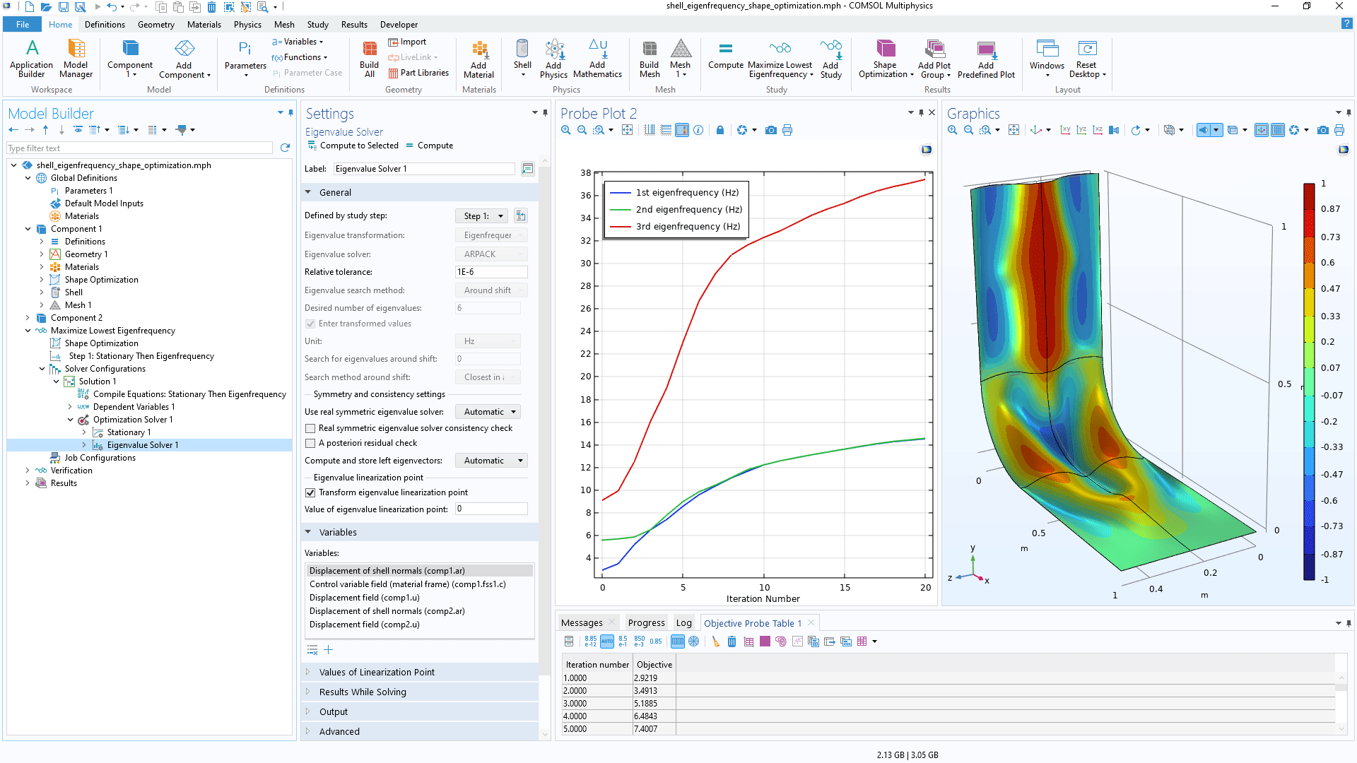
A new Stationary Then Eigenfrequency study step allows for consecutively solving a Stationary and an Eigenfrequency study in a single study step. This functionality, by default, uses the Stationary Solver to solve the dependent variables associated with the shape and topology optimization interfaces and uses the Eigenfrequency Solver to solve the dependent variables associated with the physics interfaces. This functionality is generally applicable and could be used to maximize the lowest eigenfrequency for an application in structural mechanics or to design band gaps. Note that the new Stationary Then Eigenfrequency study step solves for different sets of dependent variables in the stationary and eigenfrequency solvers, making it unsuitable for the maximization of, for example, buckling loads.
Parameter Estimation
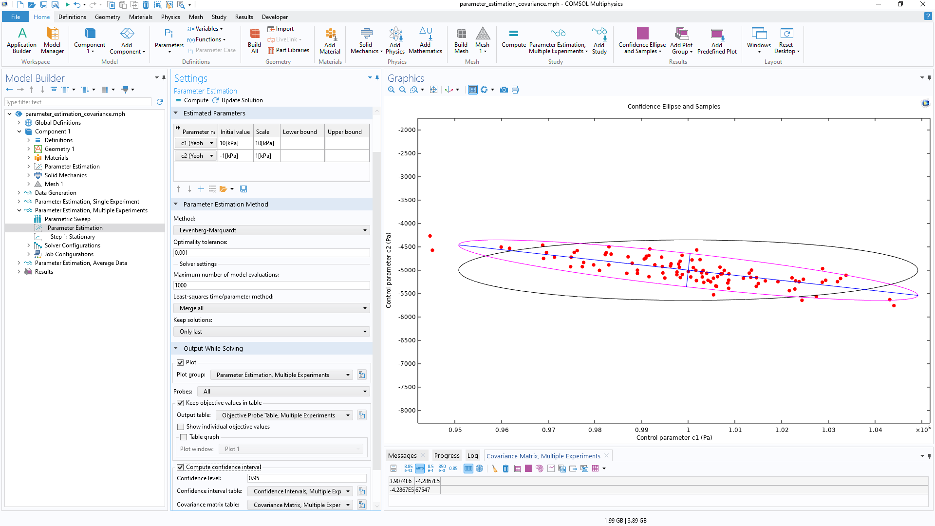
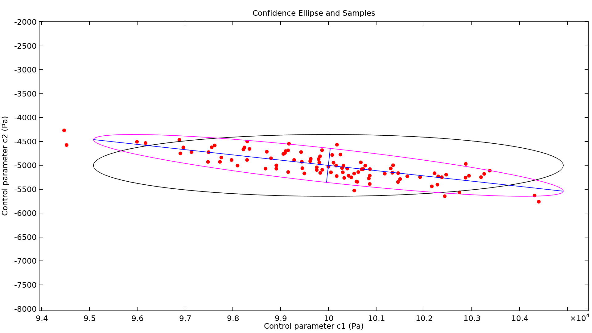
The Global Least-Squares Objective feature and the Parameter Estimation study step now provide a Variance column for specifying the variance of individual measurements. Alternatively, the variance can be estimated automatically, and, in either case, the results can be used to estimate the uncertainty of the output from parameter estimation. The simplest approach is to compute confidence intervals for the estimated parameters, but the resulting intervals may be inapplicable if the parameters are correlated. Therefore, the ability to export the covariance matrix has been added and is available with the Levenberg-Marquardt optimization method. This capability provides a more detailed assessment of output uncertainty than using the confidence intervals of the estimated parameters. Additionally, support for bounds has been added to the Levenburg-Marquardt optimization method, and this can improve robustness for nonlinear models.
Topology and Shape Optimization Updates
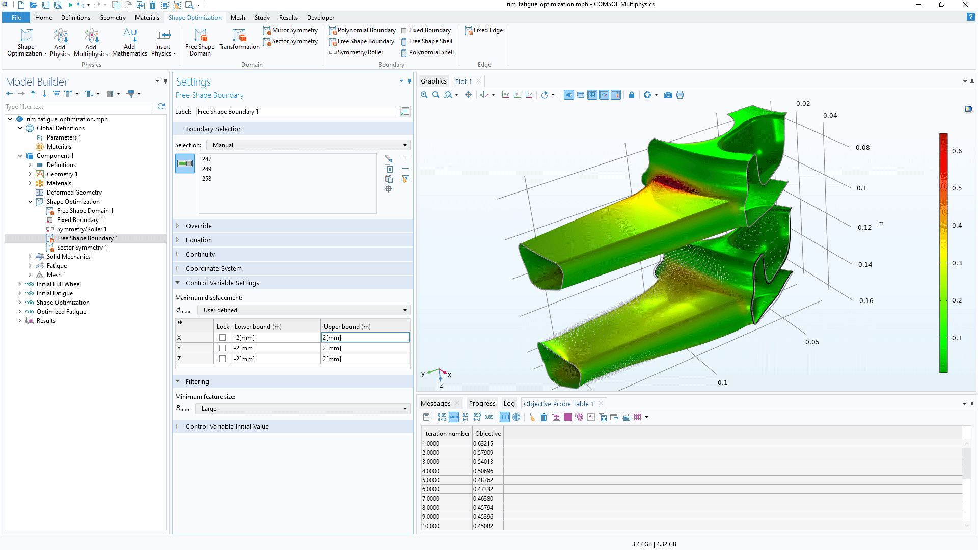
For topology optimization, new Mirror Symmetry and Sector Symmetry features have been added to simplify the setup of models where a symmetric design is required but where the effects of certain physics phenomena are not expected to be symmetric. In some cases, these features can be used to reduce the number of solutions or load cases per iteration, leading to improved performance. Additionally, the shape optimization features now include the ability to set the maximum displacement for individual components, and it is also possible to enforce a Euclidean interpretation of the maximum displacement, instead of the previous taxicab (box-like) interpretation.
General Purpose Updates
- The Control Variable Field feature includes support for grouping adjacent entities using the new geometric constant discretization.
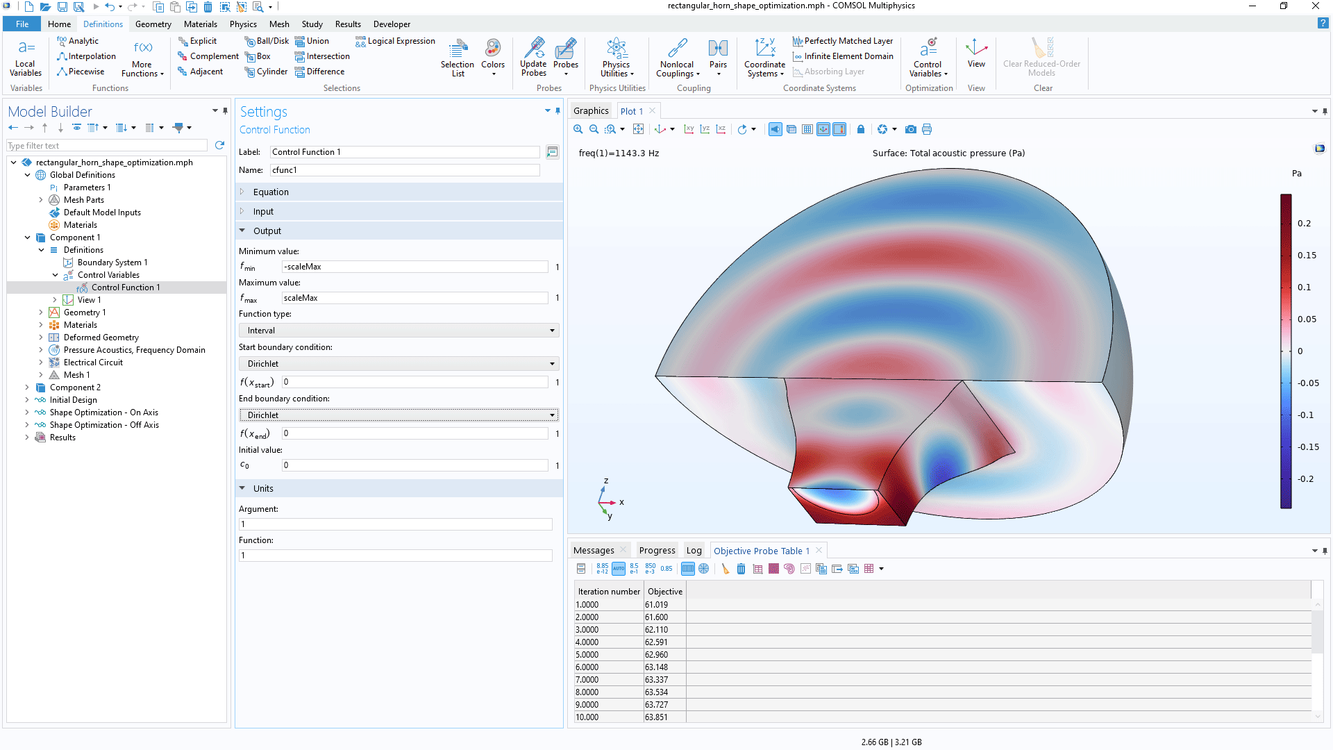
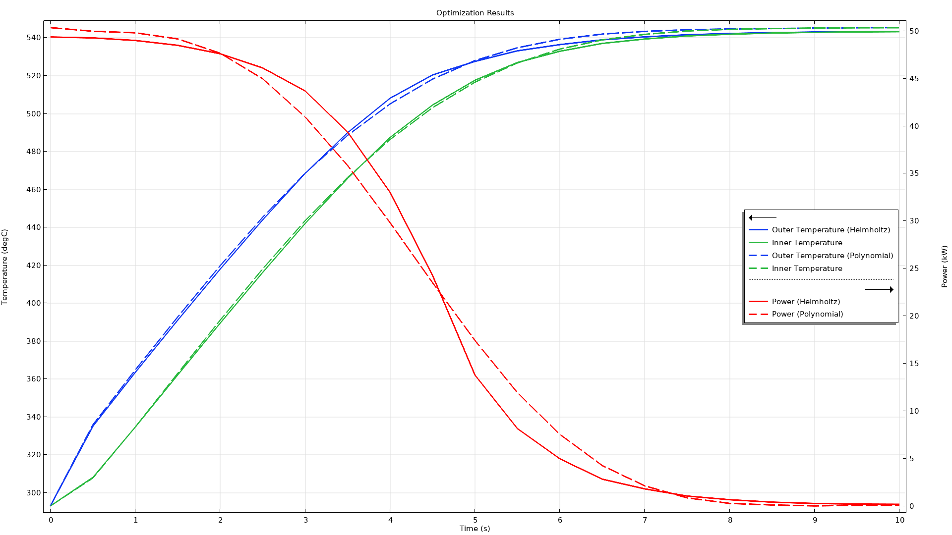
- The settings for the Control Function feature include additional options and improved consistency between polynomial functions and Helmholtz regularization.
- New Shape Optimization, Topology Optimization, and Parameter Estimation ribbon tabs appear when the features are in use, providing better consistency with the Model Builder tree.
- The Control Function and Control Variable Field features have been moved to the Definitions branch in the Model Builder tree.
New and Updated Tutorial Models
COMSOL Multiphysics® version 6.2 brings several new and updated tutorial models to the Optimization Module.
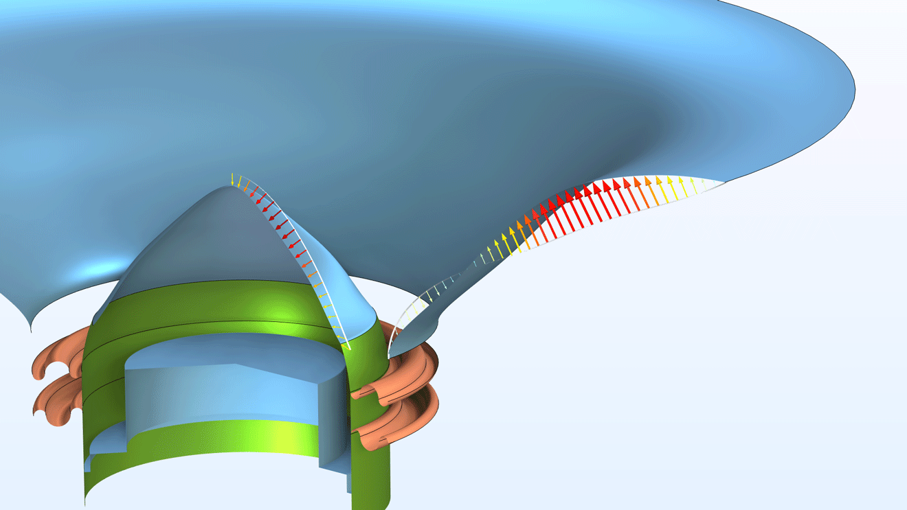
Tweeter Dome and Waveguide Shape Optimization
Application Library Title:
tweeter_shape_optimization
Download from the Application Gallery
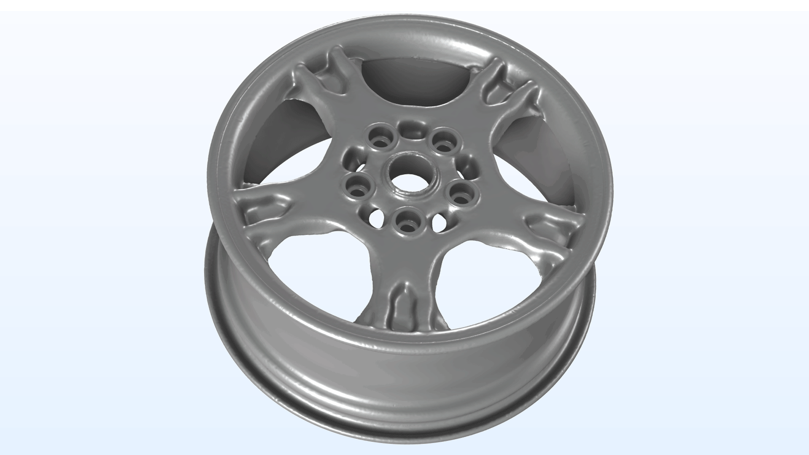
Wheel Rim — Stress Optimization with Fatigue Evaluation
Application Library Title:
rim_fatigue_optimization
Download from the Application Gallery
Wheel Rim — Topology Optimization with Milling Constraints
Application Library Title:
wheel_topology_optimization_milling
Download from the Application Gallery
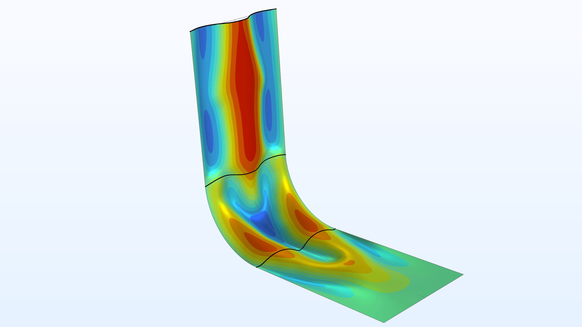
Maximizing the Eigenfrequency of a Shell
Application Library Title:
shell_eigenfrequency_shape_optimization
Download from the Application Gallery
Optimal Control for Heating of a Rod
Application Library Title:
optimal_heating_control
Download from the Application Gallery
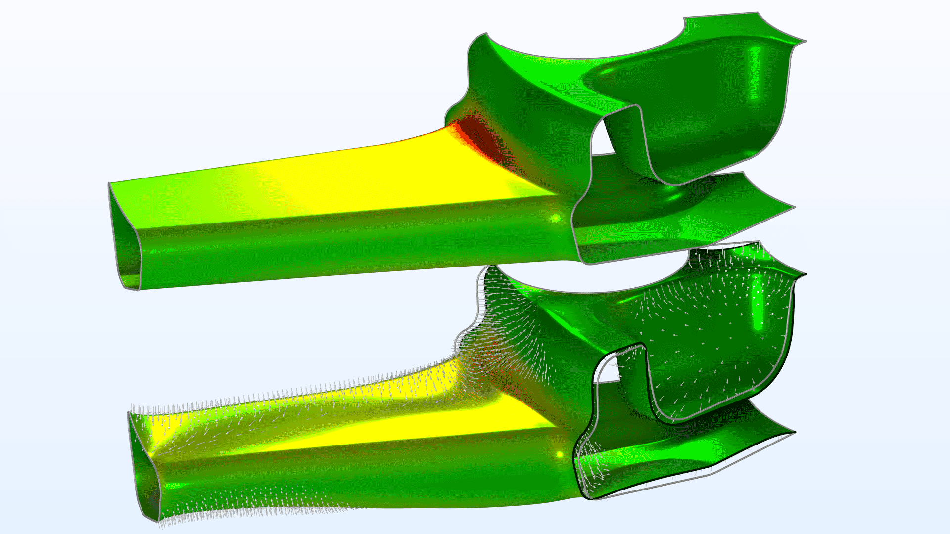
Optimization of a Waveguide Iris Bandpass Filter — Transformation Version
Application Library Title:
waveguide_filter_optimization_transformation
Download from the Application Gallery
Optimization of a Photonic Crystal for Signal Filtering
Application Library Title:
photonic_crystal_filter_optimization
Download from the Application Gallery
Maximizing the Eigenfrequency of a Beam
Application Library Title:
beam_eigenfrequency_topology_optimization
Download from the Application Gallery
Bracket — Eigenfrequency Shape Optimization
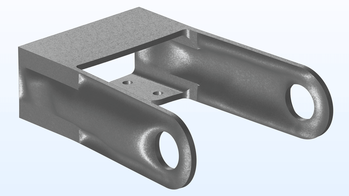
Application Library Title:
bracket_eigenfrequency_shape_optimization
Download from the Application Gallery
Ten-Bar Truss Optimization
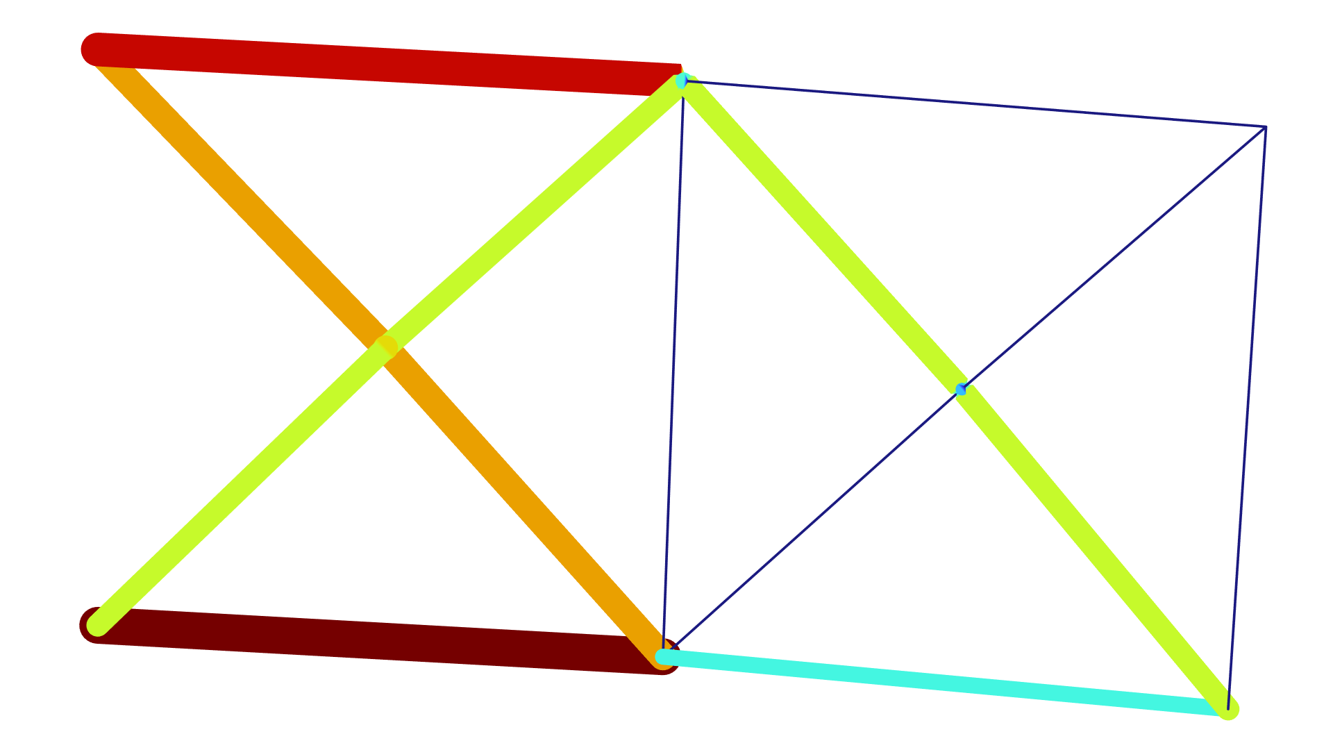
Application Library Title:
ten_bar_truss
Download from the Application Gallery
Parameter Estimation with Covariance Analysis*
Application Library Title:
parameter_estimation_covariance
Download from the Application Gallery
*Requires the Nonlinear Structural Materials Module