

Simulation apps, as we’ve highlighted on the blog, are a powerful tool for hiding complex physics behind an easy-to-use, intuitive interface. While the app can be used by those with little simulation expertise, understanding the layers beneath its interface — the embedded model and underlying theory — does require a good understanding of COMSOL Multiphysics and the physics at hand. Let’s explore the connection between theory, model, and app using the example of analyzing buckling in a truss tower design.
The Multiple Layers of a Simulation App
To help extend simulation capabilities to a wider audience, numerical modeling apps are designed with simplicity and ease-of-use in mind. While the interface that users interact with appears this way, there are many other important layers to consider behind an app’s design. The underlying theory and the embedded model, for instance, are crucial elements, as they help to ensure accuracy in the simulation results obtained by users.
So how do we connect the dots between these different elements — the theory, the model, and the app? Today, we’ll demonstrate this relationship by looking at the theory and model behind our Linear Buckling Analysis of a Truss Tower app. While an app sometimes merely embeds a model and places a simplified user interface (UI) on it, this case involves using an app to generate an advanced extension of the built-in functionality available in COMSOL Multiphysics.

Linear Buckling Analysis of a Truss Tower demo app.
The Underlying Problem: Buckling in a Truss Tower
To begin, let’s focus on the problem that the app is designed to study: buckling. If a tall vertical structure is subject to an increasing compressive load, deformations will be very small until the critical value of the load is reached. If the load is slightly increased after this point, the structure can suddenly collapse. My colleague Henrik Sönnerlind discussed this phenomenon, known as buckling, in an earlier blog post. Here, we will focus on buckling as it specifically relates to a truss tower design.
Truss towers are slender structures that can face the risk of buckling. In this model, we will consider the effects of the weight of the truss structure itself, the tension effects of the optional guy wires, and a concentrated vertical force at the top. The latter is the “payload”, typically large antennas.
From the viewpoint of buckling, a load can be considered live or dead. A dead load, like the self-weight, has a fixed value. The live load, the weight of the antenna in this case, is the load against which we want to compute the safety factor.
COMSOL Multiphysics does not include a built-in setup for solving this problem that allows us to distinguish between the live load, gravity, and wire tension effects. But with some understanding of the theory behind buckling and how the software works, such a study can be set up. We will have to write some extra equations, weak contributions as they are more often called, which are simple to incorporate into the model. This represents an important strength of COMSOL Multiphysics: Users can adjust and extend the capabilities of available features by modifying the existing implementation or writing new mathematical terms.
The tower that we will consider has a rectangular cross section with four vertical bars at the corners. Three types of members — longitudinal, transverse, and diagonal — form the tower structure. The guy wires, which are attached to the tower at two different levels, give the structure greater stiffness to protect it against, for instance, wind loads. Note that the wires are under pretension, otherwise they would not provide any stiffness. The bottom part of the truss is pinned to the ground. The screenshot below depicts the model tree structure for the buckling analysis.
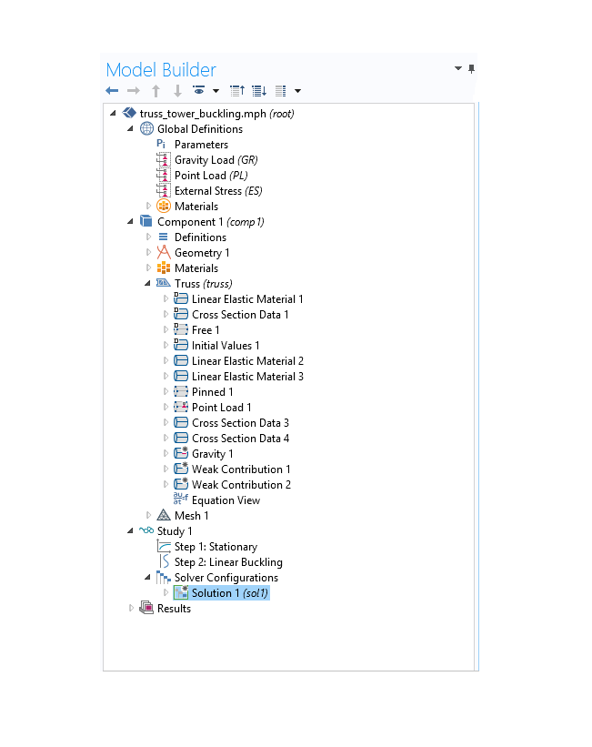
Model tree settings for the truss tower buckling analysis.
The nodal labels in the above diagram are self-explanatory:
- Linear Elastic Material 1 specifies the material properties of the truss elements
- Linear Elastic Material 2 and Linear Elastic Material 3 relate to the material properties of the guy wires
- External Stress specifies pretension in the guy wires
- Gravity considers the weight of the truss members and guy wires
- Point Load allows us to apply the vertical load on the truss tower
- Weak Contribution 1 and Weak Contribution 2 enable us to add in extra mathematical terms
Understanding Buckling Equations
Study 1 in the model tree is a predefined buckling analysis study that is included in the Truss interface and consists of two individual study steps. The first is a stationary study step in which you compute the state of stress in a structure for a given load. The second study step allows you to solve an eigenvalue problem to determine the critical load as a multiple of the load you applied. In a typical analysis of a structure, we are interested in identifying the nodal displacements due to a load \mathbf f_0 acting on it. If we put all of the nodal displacements in a vector $$\mathbf{u}_0$$ and if the structure stiffness matrix is \mathbf K, then this amounts to solving a system of equations of the form
The stiffness matrix \mathbf K can be split into linear and nonlinear parts. Thus, \mathbf K = \mathbf K_{L} + \mathbf K_{NL} (\mathbf f_0), where \mathbf K_{L} is the linear part and \mathbf K_{NL} is the extra contribution caused by considering geometric nonlinearity. Note that the nonlinear part of the stiffness matrix depends on the applied load. In a linear buckling analysis, we assume that the nonlinear part of the stiffness matrix is a linear function of the load (i.e., \mathbf K_{NL}(\lambda \mathbf f_0) = \lambda\mathbf K_{NL}(\mathbf f_0), where \lambda is a scalar multiplier). When the structure buckles, the deformation is unbounded. Numerically, this manifests itself in a singular stiffness matrix, so we must solve for the value of $\lambda$ that renders the matrix singular.
In other words, we solve the eigenvalue problem defined above. The smallest eigenvalue $\lambda_0$ is the critical load factor, and the corresponding eigenvector \mathbf u defines the buckled shape.
Now, let’s try to understand the current problem with respect to the theory explained above. Remember our assumptions? We want to include the weight of the tower and cables, as well as the pretension in the wires, in the analysis. These loads, however, do have fixed values so that their contribution to the nonlinear stiffness matrix should not be scaled by \lambda. Therefore, we are interested in solving a modified eigenvalue problem:
where \mathbf K_{NL,d}(\mathbf f_d) captures the effect of the dead loads. The eigenvalue step in the buckling study, however, only allows you to solve the standard buckling problem where all loads are considered as live loads. To change this in order to accomplish our goals, we need to look at additional mechanisms that COMSOL Multiphysics offers.
Setting Up the Linear Buckling Analysis Problem in COMSOL Multiphysics
The first step in solving our problem is to perform a stationary analysis to isolate the stiffness due to dead loads. Once this is done, we can manipulate the eigenvalue solver to include the effects of the dead loads in the problem. The plan is to solve three stationary problems, respectively, in succession:
- Solve for gravity effects and pretension
- Consider the effects of pretension in the guy wires only
- Analyze the combined effects of live weight and wire pretension
We must include the wire pretension in all static load cases. Without it, the wires have no stiffness, so the problem would be singular. As such, it is not possible to directly create a load case containing only the live weight.
To solve three different load conditions within one single stationary study step, we can group them as load groups and define appropriate load cases within the solver. In the example below, we have created three load groups: Gravity Load, Point Load, and External Stress. These groups correspond to gravity, point load, and stresses in the wires, respectively. To create these load groups, simply right-click on the Global Definitions node in the model tree and select Load Group. This generates a new load group for you, the name of which you can adjust as needed. Say you want to include the gravity node under the load group Gravity Load. In that case, simply right-click on the node and choose the Gravity Load option under Load Group.
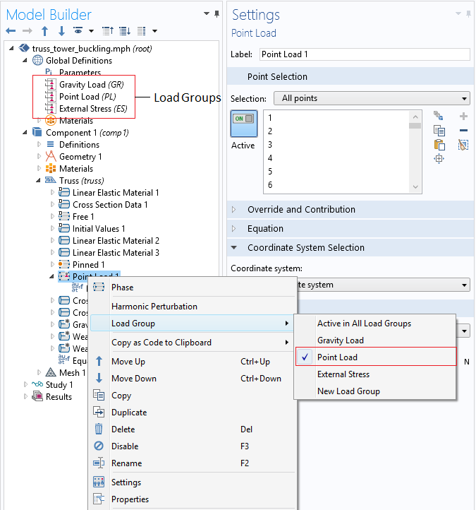
Defining load groups and grouping load types.
The reason for adding these load groups will be clear when we look at the Stationary node of Study 1. In the Study Extensions section, we can define a number of load cases to create several different stationary analyses within the same study step. In the following screenshot, three load cases are defined:
- Dead Load 1: Gravity (GR) and pretension in wires (ES)
- Dead Load 2: Pretension in wires (ES)
- Live Load: Point load acting on the tower (PL) and pretension in wires (ES)
In the case of Dead Load 1, as it may already be intuitively clear to you, the stationary solver will only solve for gravity and pretension effects, excluding the point load from the analysis. Similar considerations apply to other cases as well.
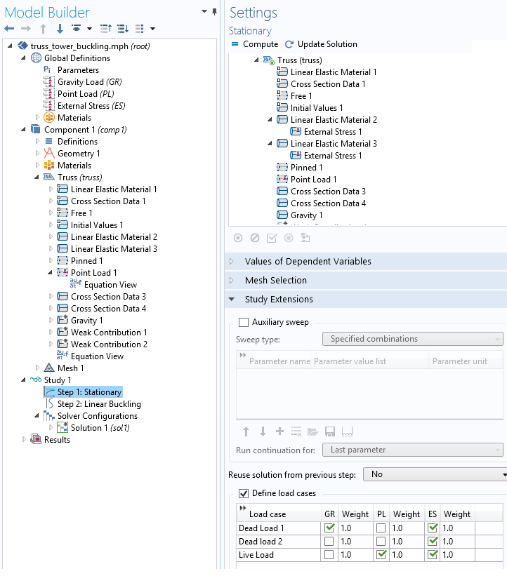
Defining load cases in the stationary solver.
Writing Weak Form Equations for the Buckling Analysis
So why we are interested in solving the stationary problem for the load cases that we just defined? We want to compute nonlinear stiffness due to dead loads, which is generated by the first stationary analysis. In this case, the effects of the weight of the truss, the weight of the guy wires, and the pretension in the wires are all included. The second stationary analysis isolates the pretension effects in the wire. Note that the weight of the wire is excluded in this step. These results are then used to eliminate the effects of guy wire pretension in the eigenvalue solver. In other words, we are solving the original problem as
where \mathbf K_{NL}^{i}, \; i=1, 2, 3 denotes the nonlinear stiffness matrix coming from the solutions of the corresponding load case scenarios. With the assumption of linearity in the nonlinear stiffness matrix contributions, this is exactly the problem that we want to solve.
To get the extra stiffness contributions, we must manually enter two terms via the Weak Contribution 1 and Weak Contribution 2 nodes. It is important to note that these weak contributions should be active only during the eigenvalue solver stage of the problem, not during the stationary study. This can be controlled in the settings for the individual study steps.
The next step involves understanding what to write in the fields of these nodes. In the case of geometric nonlinearity, the basic truss equation is
where $$Y$$ is the Young’s modulus, $$A$$ is the cross-sectional area, and \hat{u} is the displacement. As the formatting of the dependent and independent variables emphasizes, the equations are written in local directions. The equation above is the so-called strong form equation of truss. The corresponding weak form is given by the expression
where $$S$$ is the axial stress and E is the axial strain. The symbol \delta denotes variation and is represented by the test() operator in COMSOL Multiphysics. This is the type of expression that COMSOL Multiphysics understands, and it uses it to generate the stiffness matrix. In fact, if you go to the Equation View of Linear Elastic 1, you will see the same expression written under Weak Expressions, as highlighted below.
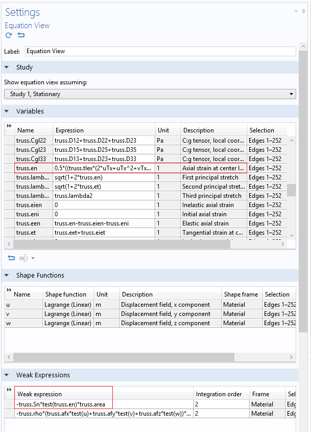
Axial strain and weak expression for the truss tower model.
The expression for the strain, truss.en, can actually have two different values,
0.5*((truss.tlex*(2uTx+uTx^2+vTx^2+wTx^2)+truss.tley*(vTx+uTy+uTy*uTx+vTy*vTx+wTy*wTx)+

truss.tlez*(wTx+uTz+uTz*uTx+vTz*vTx+wTz*wTx))*truss.tlex+

(truss.tlex*(vTx+uTy+uTy*uTx+vTy*vTx+wTy*wTx)+truss.tley*(2vTy+uTy^2+vTy^2+wTy^2)

+truss.tlez*(wTy+vTz+uTz*uTy+vTz*vTy+wTz*wTy))*truss.tley+

(truss.tlex*(wTx+uTz+uTz*uTx+vTz*vTx+wTz*wTx)+truss.tley*(wTy+vTz+uTz*uTy+vTz*vTy+wTz*wTy)+

truss.tlez*(2wTz+uTz^2+vTz^2+wTz^2))*truss.tlez)
or
(uTx*truss.tlex+0.5*truss.tley*(vTx+uTy)+0.5*truss.tlez*(wTx+uTz))*truss.tlex+

(0.5*truss.tlex*(vTx+uTy)+truss.tley*vTy+0.5*truss.tlez*(wTy+vTz))*truss.tley+

(0.5*truss.tlex*(wTx+uTz)+0.5*truss.tley*(wTy+vTz)+truss.tlez*wTz)*truss.tlez
The first expression is the one you would see in the case of a geometrically nonlinear study. The latter strain expression is much simpler, as it is for a geometrically linear case.
Now the plan of action is simple. The linear terms of stiffness \mathbf K_L are independent of the loads and they are automatically included in the analysis. To include the nonlinear stiffness matrix due to dead loads, we should extract the stresses from the first stationary analysis and multiply this by the test of only the nonlinear part of the strain function. The stress from the first stationary analysis can be obtained with the withsol() operator in COMSOL Multiphysics. This gives us the following expression that goes in the Weak Contribution 1 node.
-withsol(sol2,truss.Sn,setval(loadcase,1))*test(0.5*

((truss.tlex*(uTx^2+vTx^2+wTx^2)+truss.tley*(uTy*uTx+vTy*vTx+wTy*wTx)+truss.tlez*(uTz*uTx+vTz*vTx+wTz*wTx))*truss.tlex

+(truss.tlex*(uTy*uTx+vTy*vTx+wTy*wTx)+truss.tley*(uTy^2+vTy^2+wTy^2)+truss.tlez*(uTz*uTy+vTz*vTy+wTz*wTy))*truss.tley

+(truss.tlex*(uTz*uTx+vTz*vTx+wTz*wTx)+truss.tley*(uTz*uTy+vTz*vTy+wTz*wTy)+truss.tlez*(uTz^2+vTz^2+wTz^2))*truss.tlez))*truss.area
A similar expression is used to exclude the effects of guy wire stresses from the eigenvalue analysis. Note that the expression there is multiplied with a $$\lambda$$ at the end. Further note that the stresses from the second stationary analysis are accessed via the withsol() operator. The argument of the setval() function is changed to 2. Now if you click the Compute button, you should get the correct critical load for the truss tower design.
The Underlying Theory and Physics Behind a Numerical Modeling App
Numerical modeling apps are comprised of various layers. Behind an app’s simplified user interface is an embedded model and underlying theory that helps to ensure both accuracy and efficiency in simulation results. Here, we have highlighted this in the case of an app developed to analyze linear buckling in a truss tower design. As the example shows, the combined flexibility of COMSOL Multiphysics and the Application Builder is powerful in addressing complex problems, fostering efficiency at every step of the design process.
Learn More About How to Develop and Design Simulation Apps
- Already building apps of your own?
- Browse additional blog posts relating to simulation apps for further inspiration and guidance
- Looking to get started?
- Watch this video for a quick introduction on turning your COMSOL models into apps
- Attend a free workshop to get hands-on experience


Comments (0)