Heat Transfer Module
New App: Heat Sink with Fins
This new app includes the geometry of a heat sink that is parameterized and considers conjugate heat transfer, where the fluid flow is modeled using the algebraic yPlus turbulence model. The model can simulate different heat sink widths and fin dimensions at arbitrary cooling air velocities. Even the number of heat sinks can be varied.
The output gives the cooling power and the average pressure drop over the length of the system. The more fins that are added, the higher the cooling power, but the pressure drop over the heat sink increases accordingly.
 Application interface showing the velocity profile obtained via the user settings.
Application interface showing the velocity profile obtained via the user settings.
New App: Concentric Tube Heat Exchanger Dimensioning Tool
In this brand new simulation app, a heat exchanger made of two concentric tubes contains two fluid domains at different temperatures. The Non-Isothermal Flow multiphysics interface is used to model heat transfer in the heat exchanger. This application computes quantities that characterize the heat exchanger, such as exchanged power, pressure drop, and effectiveness. The pipe structure, fluid properties, and boundary conditions are all customizable.
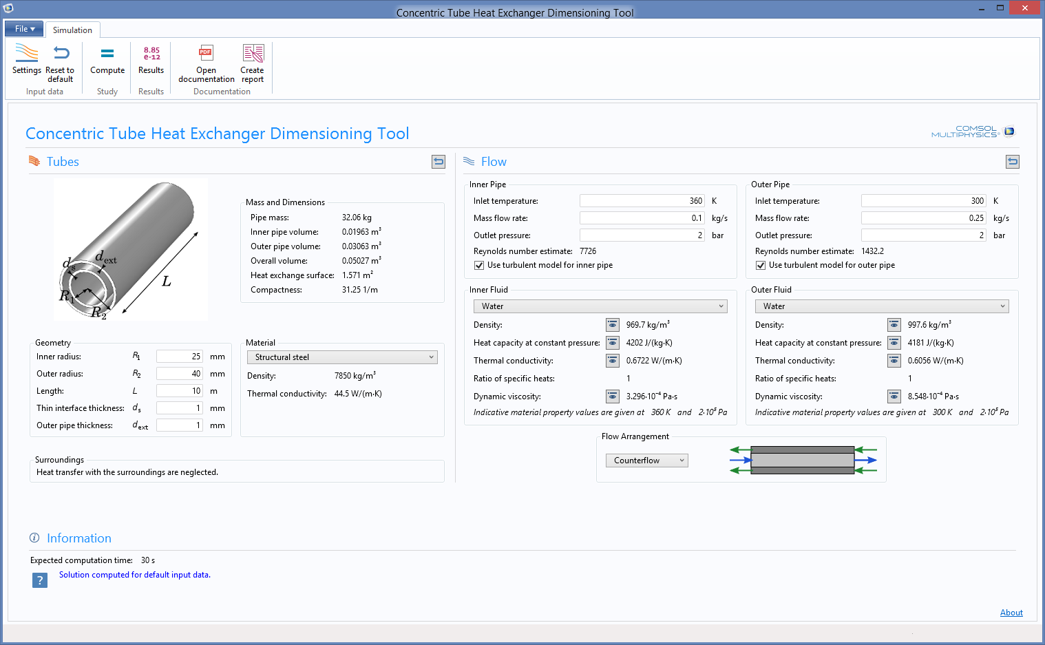 Defining the properties of the tubes in the Concentric Tube Heat Exchanger App.
Defining the properties of the tubes in the Concentric Tube Heat Exchanger App.
Algebraic Turbulence Models
The algebraic turbulence models yPlus and L-VEL are now available in the Heat Transfer Module. These enhanced viscosity models are suitable for interior flows such as those in electronic cooling applications. The algebraic turbulence models are computationally less expensive and more robust, but generally less accurate than transport equation models like the k−ε model. These turbulence models are available in Single-Phase Flow interface and in the multiphysics interfaces Non-Isothermal Flow and Conjugate Heat Transfer.
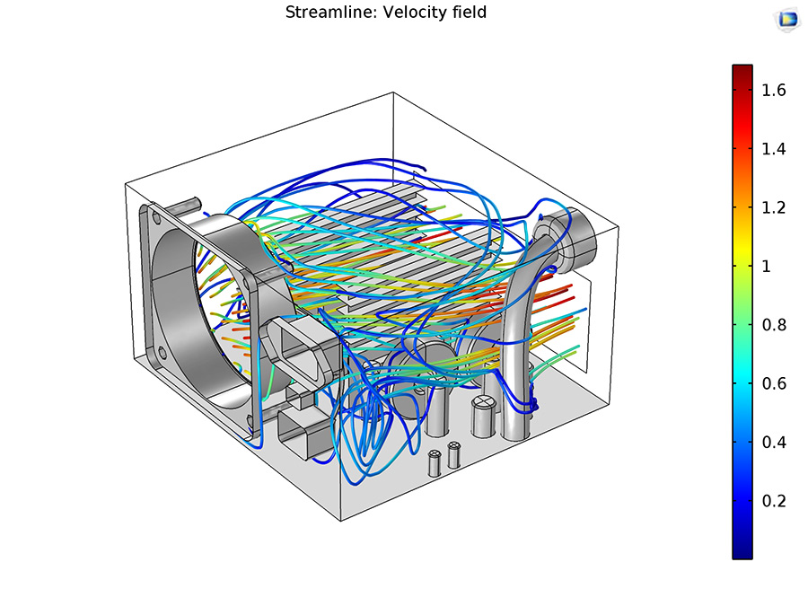 Streamlines computed using the yPlus algebraic turbulence model in a power supply unit (PSU).
Streamlines computed using the yPlus algebraic turbulence model in a power supply unit (PSU).
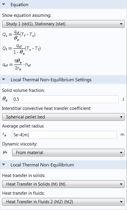
Local Thermal Non-Equilibrium Multiphysics Interface
The Local Thermal Non-Equilibrium (LTNE) multiphysics interface is designed to simulate heat transfer in porous media on the macro scale, where the temperatures in the porous matrix and the fluid are not in equilibrium. It differs from simpler macro-scale models for heat transfer in porous media where temperature differences between the solid and fluid phases are neglected. Typical applications can involve rapid heating or cooling of a porous medium using a hot fluid, or internal heat generation in one of the phases (due to inductive or microwave heating, exothermic reactions, etc.) This phenomenon is observed in nuclear devices, electronics system, or fuel cells, for example.
Coupled Porous Media Flow and Turbulent Flow
The Single-Phase Flow interfaces can now model turbulent flow in a free medium that is coupled to a porous medium. You can activate this functionality by adding a Fluid and Matrix Properties domain node for the Algebraic yPlus or L-VEL turbulence models. These turbulence models are only available in the CFD and Heat Transfer Modules, but you can still couple them to Porous media flow interfaces available in other modules.
You can either start with a porous media flow interface and add a free-flow domain or you can start with a free-flow interface and add a porous domain. The Enable porous media domains checkbox adds the Fluid and Matrix Properties feature. The Brinkman equations are solved in the porous domains and the Reynolds-averaged Navier-Stokes equations are solved in the free-flow domains.
Finally, your modeling capabilities have been extended by the fact that the Forchheimer term can be added to the equations for porous media flow. This allows for the description of high interstitial velocities (i.e., high velocities in the pores).
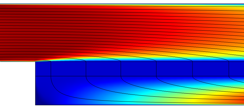
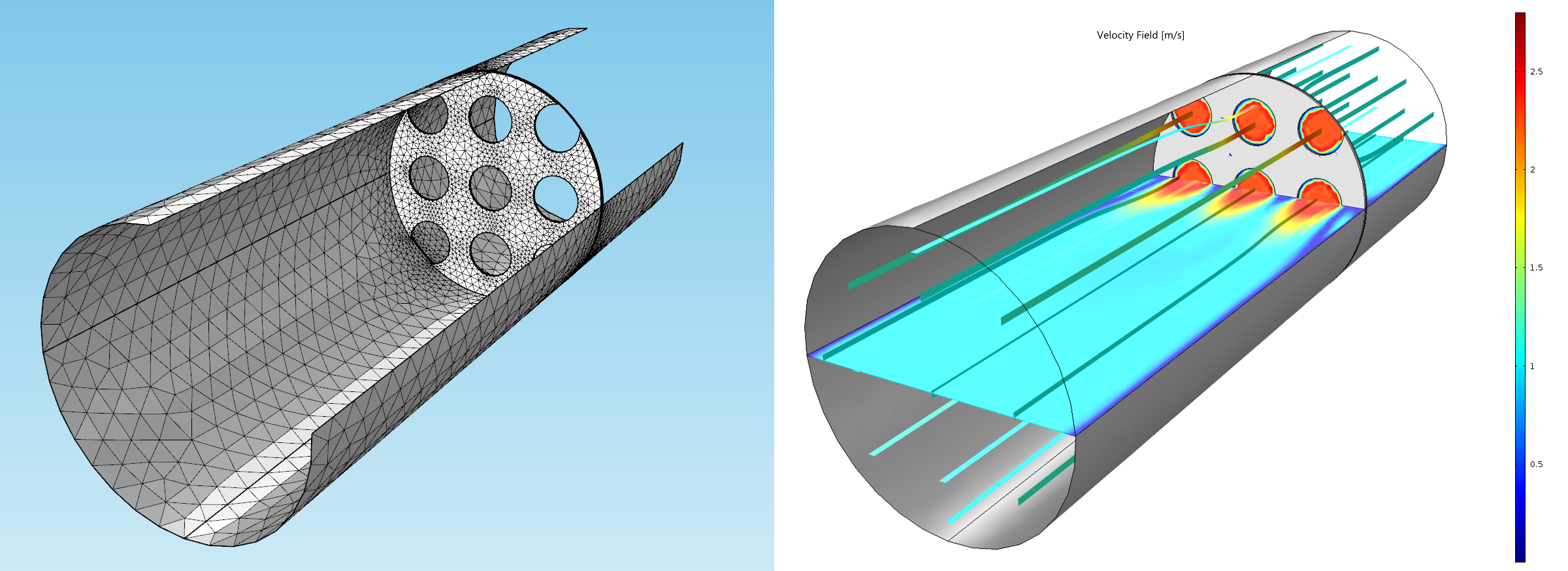 This figure shows a porous filter, furthest away from the viewer, supported by a perforated solid plate. A flow is pumped through the filter, where the effect of the porous filter and the perforations in the supporting plate on the turbulent flow are automatically accounted for in the flow interface.
This figure shows a porous filter, furthest away from the viewer, supported by a perforated solid plate. A flow is pumped through the filter, where the effect of the porous filter and the perforations in the supporting plate on the turbulent flow are automatically accounted for in the flow interface.
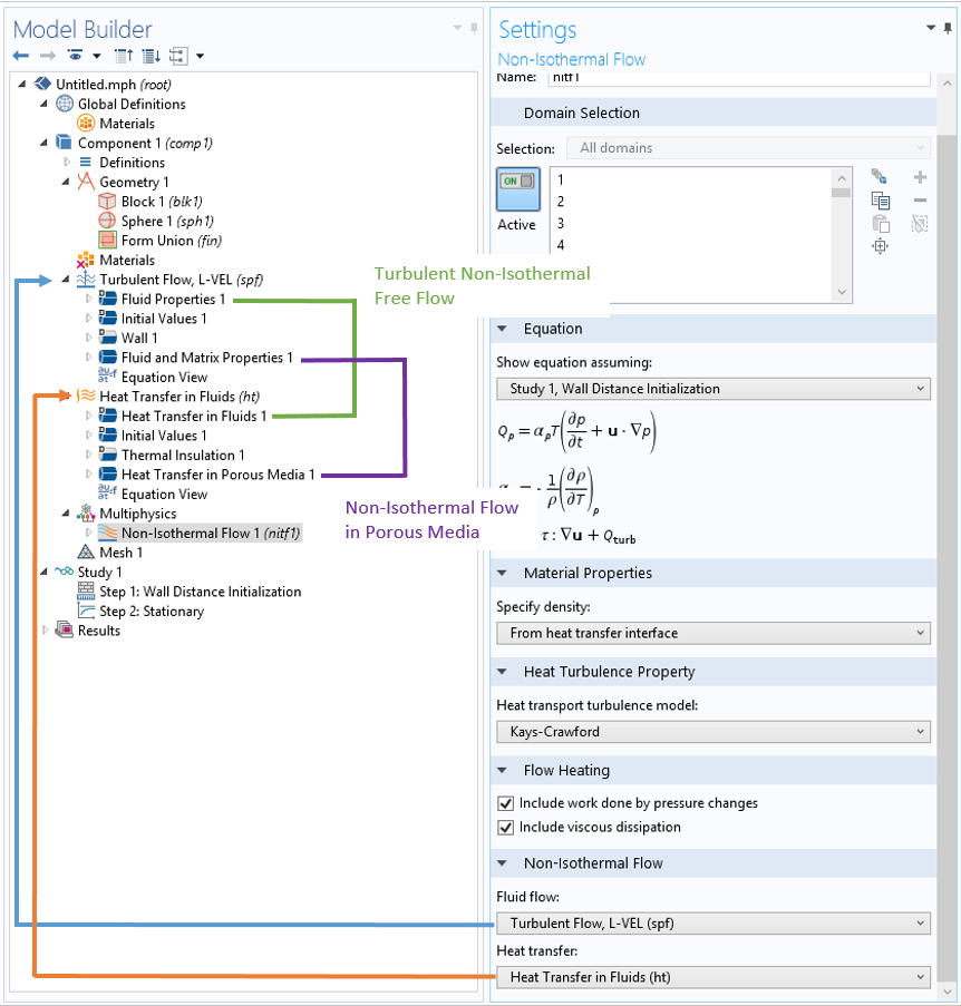
Non-Isothermal Flow Coupling in Porous Domains
A Fluid and Matrix Properties feature has been introduced in the Single Phase Flow interface in COMSOL Multiphysics 5.1 in the following modules: Batteries and Fuel Cells, CFD, Chemical Reaction Engineering, Corrosion, Electrochemistry, Electrodeposition, Microfluidics, and Subsurface Flow.
In parallel, the Non-Isothermal Flow multiphysics coupling node, which is found in the Heat Transfer Module and CFD Module, has also been updated. It can now simulate multiphysics phenomena that require the coupling to the Heat Transfer in Porous Media and the Fluid and Matrix Properties features.This capability can be used to model non-isothermal flow in porous media, such as natural convection occurring due to a variable temperature distribution through a porous medium's matrix. The viscous dissipation and the work done by pressure forces can also be solved for in porous media domains.
Furthermore, it is possible to use the Non-Isothermal Flow multiphysics coupling node to simulate non-isothermal turbulent flow. This is done by using the algebraic turbulence model in the free domains and coupling to porous media flow over the interface.
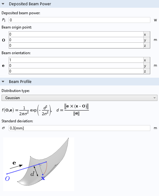
Deposited Beam Power
The new Deposited Beam Power feature is available in 3D and is used to model narrow laser, electron, or ion beams that deposit power on a localized spot. The user interface provides different options to define the beam properties and profile type: Gaussian or Top-hat disk. It also allows for the definition of the beam origin point, its direction vector, its thickness, and the deposited power. From these inputs, the Deposited Beam Power feature determines the intersection point with the selected boundaries, and a localized heat source is applied according to the selected distribution function.
Marangoni Effect
A new boundary multiphysics feature couples the single-phase flow and heat transfer interfaces, to model the Marangoni effect induced by a temperature-dependent surface tension. Marangoni (or thermo-capillary) convection occurs when the surface tension of an interface (generally liquid-air) depends on the temperature. This is of primary importance in the fields of welding, crystal growth, and the laser or electron beam melting of metals.
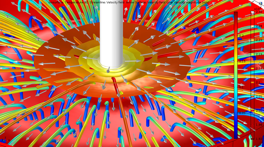 Isothermal surfaces, flow direction on the surface (arrows), and streamlines in the fluid induced by the Marangoni effect in a liquid metal heated by a laser beam.
Isothermal surfaces, flow direction on the surface (arrows), and streamlines in the fluid induced by the Marangoni effect in a liquid metal heated by a laser beam.
Optimized Default Mesh Settings for Heat Transfer Interfaces
The default mesh settings in all heat transfer interfaces utilize periodic conditions and pair conditions. When these features are enabled, the default mesh uses an identical mesh on the source and destination boundaries to minimize the numerical error induced by extrapolation, which occurs when the meshes on both sides do not coincide. In addition, the physics-controlled auto-mesh suggestion automates meshing for infinite elements. The new auto-mesh suggestion automatically applies swept (3D) or mapped (2D) meshing to domains with infinite elements.
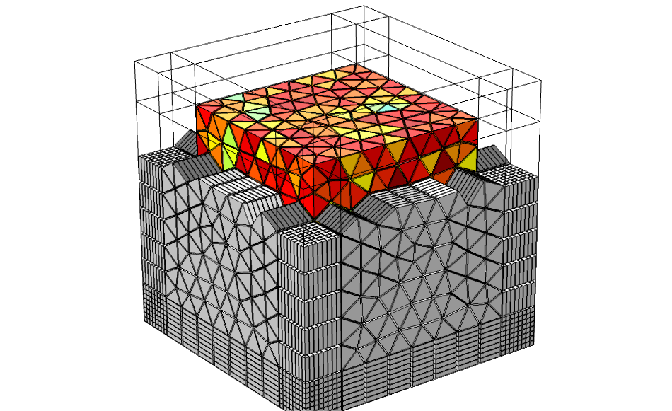 Default mesh obtained for infinite element domains (gray elements) surrounding an internal domain with arbitrary mesh (colored elements).
Default mesh obtained for infinite element domains (gray elements) surrounding an internal domain with arbitrary mesh (colored elements).
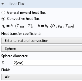
Additional Correlations for Heat Transfer Coefficients
Two convective heat transfer coefficient correlations have been added to the heat transfer coefficients library corresponding to external flow induced by natural convection, around either a sphere or a long horizontal cylinder. These heat transfer coefficients can be used to reduce the simulation cost when the model configuration corresponds to one of these situations. In these cases, the flow computation and heat convection in the fluid are replaced by a heat flux boundary condition on the solid boundaries.
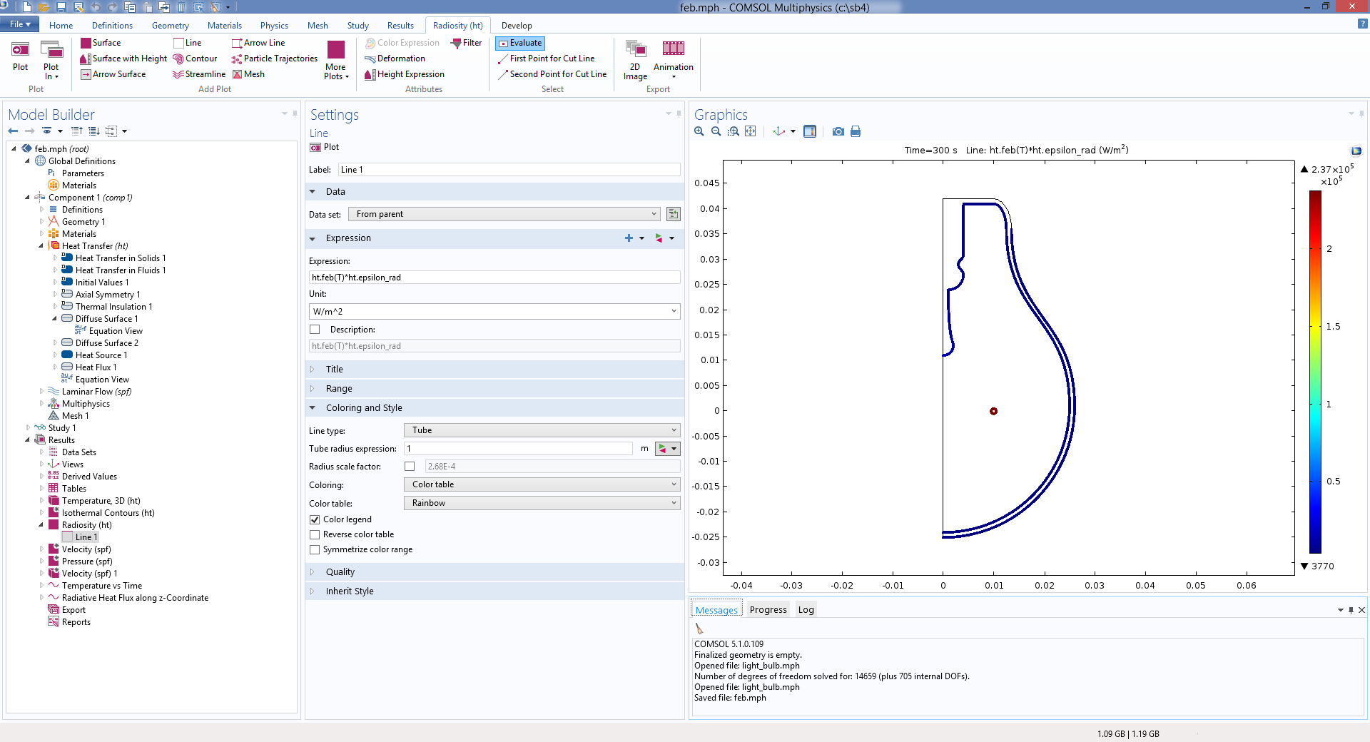
Predefined Functions for Blackbody Intensity and Blackbody Emissive Power
The heat transfer interfaces provide two new functions, ht.fIb(T) and ht.feb(T), to evaluate the blackbody intensity and the blackbody emissive power, respectively. For both functions, the refractive index of the media is accounted for. Because these quantities are defined as functions of a blackbody temperature, it is possible to evaluate them for arbitrary temperatures. For example, ht.feb(5770[K]) returns the emissive power at 5770 K, which is a temperature used to model the sun as a blackbody.
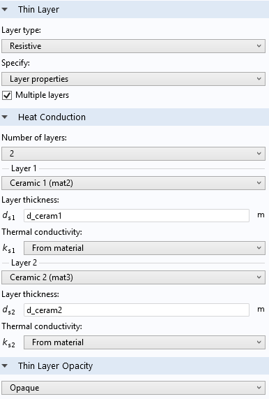
Improved Support of Thin Layer Feature
The Thin Layer boundary feature is used to model small (particularly, thin) structures that have a noticeable effect on the overall results of the model. Despite the small dimensions of the layers, the temperature may vary significantly depending on the thickness of the layers. This feature has been updated to consider other phenomena than just conduction, such as surface-to-surface boundary conditions, isothermal domains, or thermal wall functions.
Bioheating Computations Now More than Five Times Faster
For heating of biological tissue, a new solution method can give more than five times speedup. This performance improvement is available for damage integral analysis when the Temperature of threshold option is active and Temperature of necrosis reached due to hyper- or hypothermia In addition, the detection of temperatures exceeding the temperature of necrosis has been improved.
Refactored Equations Shown in Equation Section
The equations displayed in the "Equation" section of all features have been improved for better readability and consistency.
 Example of an updated equation in the Heat Transfer in Fluids feature.
Example of an updated equation in the Heat Transfer in Fluids feature.
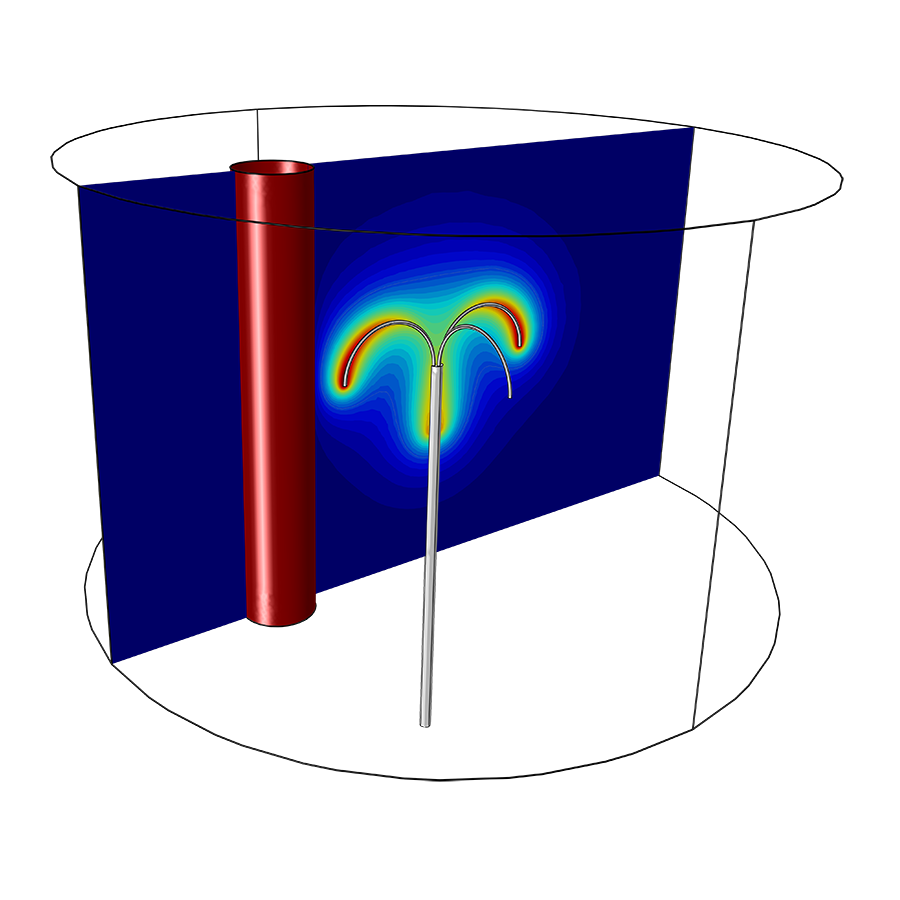
New Tutorial: Modeling a Conical Dielectric Probe for Skin Cancer Diagnosis
The response of a millimeter wave with frequencies of 35 GHz and 95 GHz is known to be quite sensitive to water content. The model in this simulation app utilizes a low-power 35 GHz Ka-band millimeter wave and its reflectivity to moisture for noninvasive cancer diagnosis.
Since skin tumors contain more moisture than healthy skin, it leads to stronger reflections on this frequency band. Hence, the probe detects abnormalities in terms of S-parameters at the tumor locations. A circular waveguide at the dominant mode and a conically tapered dielectric probe are quickly analyzed, along with the probe's radiation characteristics, using a 2D axisymmetric model. Temperature variation of the skin and the fraction of necrotic tissue analyses are performed as well.
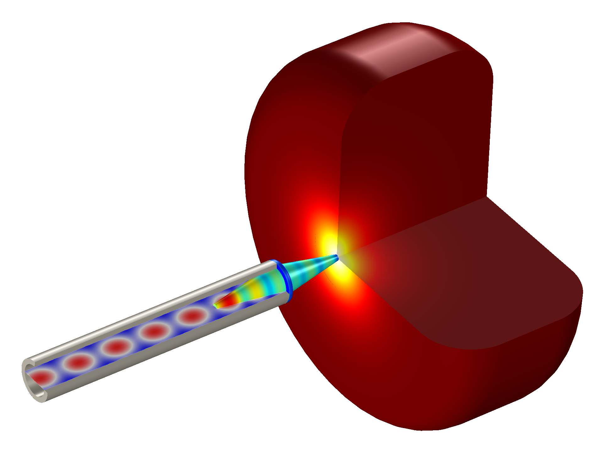 Simulation showing that the temperature variation induced by the probe radiation is less than 0.06 K even after 10 minutes of exposure.
Simulation showing that the temperature variation induced by the probe radiation is less than 0.06 K even after 10 minutes of exposure.
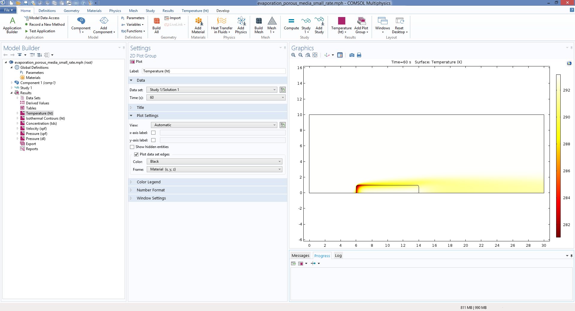
New Tutorial: Evaporation in Porous Media with a Small Evaporation Rate
Evaporation in porous media is an important process in the food and paper industries, among others. Many physical effects must be considered: fluid flow, heat transfer, and transport of the participating fluids. This tutorial model describes laminar air flow through a humid porous medium. The air is dry at the inlet and its moisture content increases as air flows through the porous medium. The evaporation rate is small enough to neglect the induced property changes in the porous medium.
Updated Tutorial: Vacuum Flask
This app calculates how much heat a vacuum flask holding hot fluid dissipates over time. It includes the recently introduced Isothermal Domain feature to monitor the temperature.
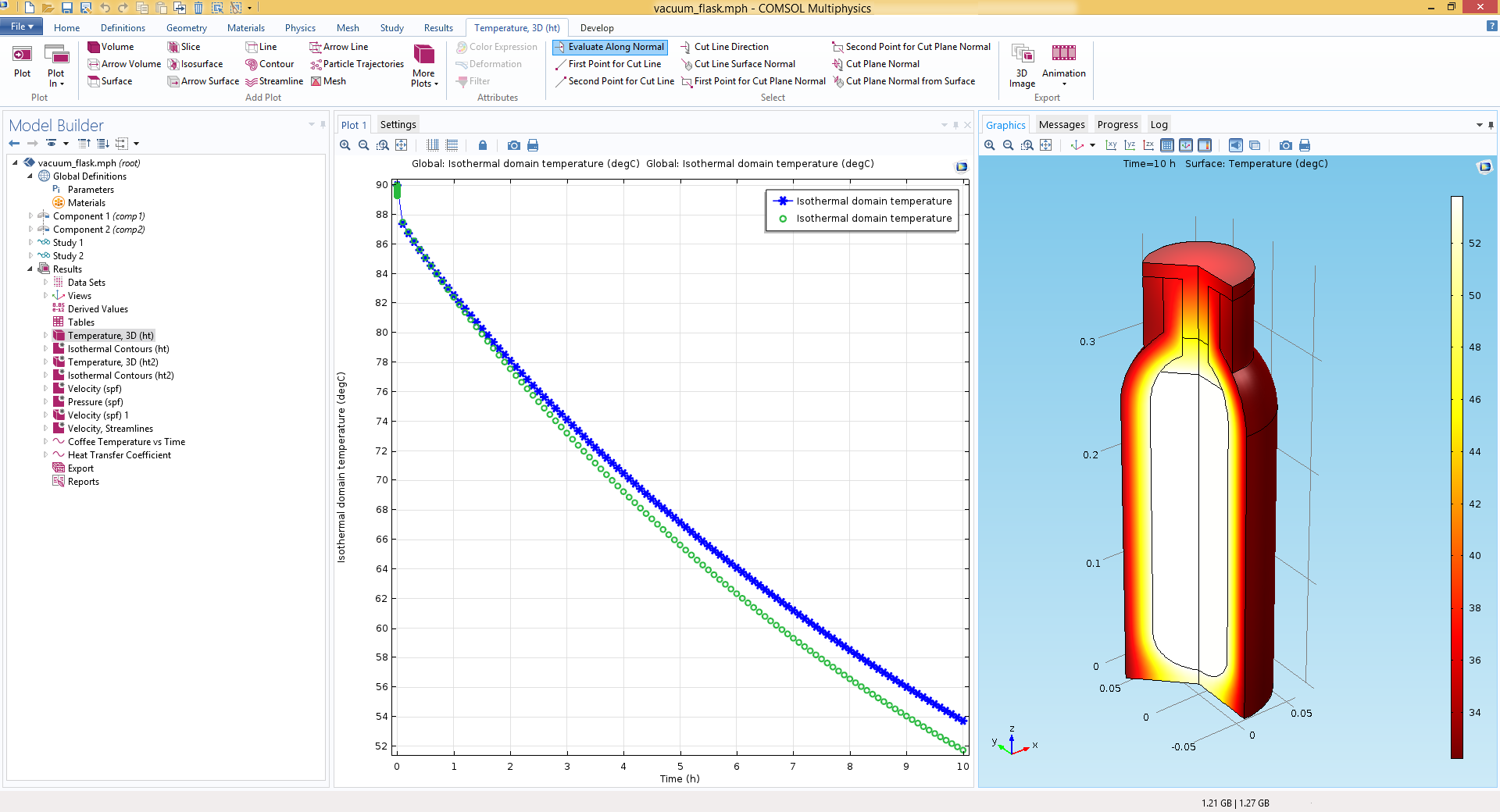 Temperature decrease of coffee (left) and the final temperature (right) profile in a vacuum flask after 10 hours.
Temperature decrease of coffee (left) and the final temperature (right) profile in a vacuum flask after 10 hours.
Updated Tutorial: Electronic Enclosure Cooling
This application uses the new yPlus algebraic turbulence model to model the flow. You can thereby model flow in the device more quickly, where the meshing and solver settings have been simplified, which also makes the model set-up faster. The application solves 1.1 MDOF and requires about 6 GB of memory for solving.
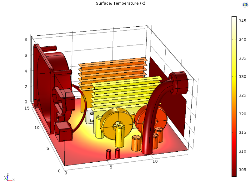 Temperature profile in a power supply unit (PSU) cooled by a turbulent flow using the new yPlusalgebraic turbulence model.
Temperature profile in a power supply unit (PSU) cooled by a turbulent flow using the new yPlusalgebraic turbulence model.
New Tutorial: View Factor Computation
This benchmark demonstrates how to compute geometrical view factors for two concentric spheres that irradiate each other. It compares simulation results to exact analytical values.
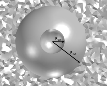 Benchmark geometrical configuration of an app that calculates geometrical view factors for two concentric spheres that irradiate each other.
Benchmark geometrical configuration of an app that calculates geometrical view factors for two concentric spheres that irradiate each other.