

One of the main issues with high-power electrical devices is thermal management. Together with BLOCK Transformatoren-Elektronik GmbH, we created a model using COMSOL Multiphysics simulation software that encompasses all of the important details when modeling heating of high-power electrical devices. To do so, we had to utilize high performance computing (HPC) with hybrid modeling. Here, we will discuss how to approach this real-life task with the COMSOL software.
Modeling Thermal Management: Test Set-Up
Our test set-up consists of a copper coil wound around a laminated iron core with some plastic and aluminum parts for stability. A conventional computer fan is placed one meter away from it. The occurring electromagnetic losses have to be calculated as well as the turbulent non-isothermal fluid flow around the device. The iron core has an air gap, which is intentionally included in order to analyze the influence it has on currents inside the coil and aluminum parts.
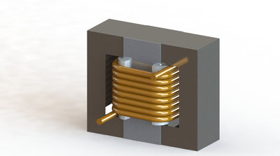
The inductor device.
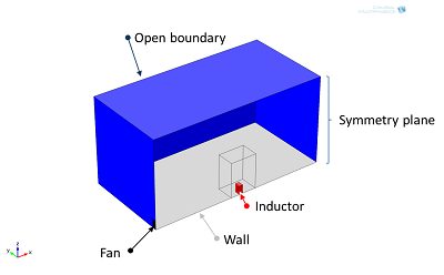
Schematic of the test set-up.
First Things First
Engineers — especially those working within project deadlines — are always looking for the right balance between computational (and modeling) efforts and accuracy. Therefore, it is a good idea to start with thinking of a suitable simplification, since the aspect ratio of the model geometry is quite challenging.
The distance between the fan and device is roughly one meter, while the interior gaps between the copper winding are about 0.1 millimeters, resulting in an aspect ratio of 10,000. In order to keep the processing time as low as possible, we choose a submodeling approach. A first model with a simplified transformer geometry is used to calculate the large-scale flow field around the device. Due to symmetry, only half of the geometry is modeled. The results of this model are exported and used as an inlet condition for the following step.
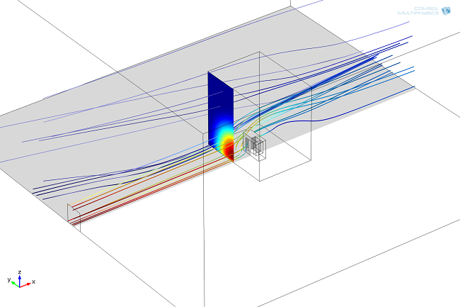
Streamline plot of the velocity field. This field was used as an inlet boundary condition in the detailed model (at the position of the slice plot).
Detailed Geometry
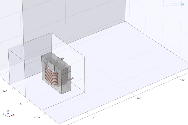
The geometry of the detailed electrical device is built in SolidWorks® software and imported into COMSOL Multiphysics® via the CAD Import Module. Only a small part is used for the non-isothermal flow calculation in the detailed submodel (about 400 mm by 900 mm). The electromagnetic part needs to be solved for an even smaller domain (200 mm by 200 mm).
Modeling the Laminated Iron Core
The iron core is laminated in order to reduce eddy currents. We’ll use the same approach as described by TU Dresden & ABB. The material is homogenized and defined with an orthotropic electrical conductivity. This allows us to keep a single domain and a coarser mesh rather than resolving the lamination geometrically with all small plates.
Electromagnetic Losses
Due to the alternating current at 500 Hz, inductive effects in the coil (skin and proximity effect) have to be resolved. Additionally, eddy currents in the aluminum plates and iron core will heat up the device.
")
Surface plot of the eddy currents in the aluminum plates. The air gap in the iron core is highlighted in red. Most currents are induced close to this gap.
")
Slice plot of the current density inside the copper coil. The air gap within the iron core is shown in red.
Due to hysteresis, there are also some magnetization losses. These are quite small in comparison to the eddy current losses and are not explicitly solved for. The table below shows the magnetization losses as functions of the magnetic flux density Qmag = f(B). We could use an interpolation function instead of solving hysteresis time-dependently.
| Part |
Electromagnetic losses |
|---|---|
| Copper coil |
37.2 W |
| Aluminum, eddy currents |
36.2 W |
| Laminated core, eddy currents |
0.02 W |
| Laminated core, magnetic losses |
0.004 W |
Velocity Field and Temperature Distribution
The device reaches a maximum temperature of 125°C on the backside of the coil.
")
Streamline plot of the velocity field and surface plot of the temperature distribution.
")
Alternative view of the velocity field.
Best Choice for Multiphysics High Performance Computing
Today, our task was to find the best solution for computing thermal designs of transformers. In the case of BLOCK Transformatoren, they decided that COMSOL Multiphysics was the most suitable for their application after comparing the handling and results of several simulation tools.
In the end, this model involved simultaneous solving for a maximum of 8 million degrees of freedom (DOFs), using a robust combination of direct and iterative solvers. Memory (RAM) usage peaked at 89 GB of memory.
In order to be able to solve highly complex models, they chose the Ready-to-Go+ (RTG+) package with a benchmarked cluster for optimal performance. With everything being set for advanced simulations at BLOCK, we can expect their products to be pushed even closer to the limit in the future.
SolidWorks is a registered trademark of Dassault Systèmes SolidWorks Corp.


Comments (0)