
Whenever you are modeling coils with the AC/DC Module in COMSOL Multiphysics, you need to consider what type of boundary conditions to use to truncate your modeling domain. In this blog post, we will introduce the different boundary conditions that you can use and how to choose between them.
Boundary Conditions for Modeling Coils: An Overview
As we introduced in our previous blog post on the basics of coil modeling, whenever you are modeling an electromagnetic coil, you need to think in terms of a closed current loop. The current loop can be entirely within the modeling domain or closed via a boundary condition, as illustrated in the figure below.
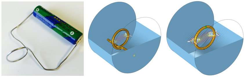
A coil connected to a voltage source (left) and two different approaches to closing the current loop (right).
As we learned earlier, if the coil extends to the boundaries of the modeling domain, then the current flowing through the coil will return along the modeling domain boundaries. Otherwise, to close the current loop, the coil must loop within the modeling domain. Here, we will concern ourselves with two questions. First, what boundary conditions should we use? And second, how far away from the coil should these boundaries be?
We will start by thinking of our coil as sitting in a space that extends to infinity and does not contain anything else. Obviously, we cannot model an infinitely large domain. We must truncate our modeling domain to some finite size that will give reasonably accurate results but will not require too much computational effort to solve. First, let us consider the case of an axisymmetric coil that is closed within the modeling domain. This case can be analyzed via a 2D axisymmetric model, as shown below.
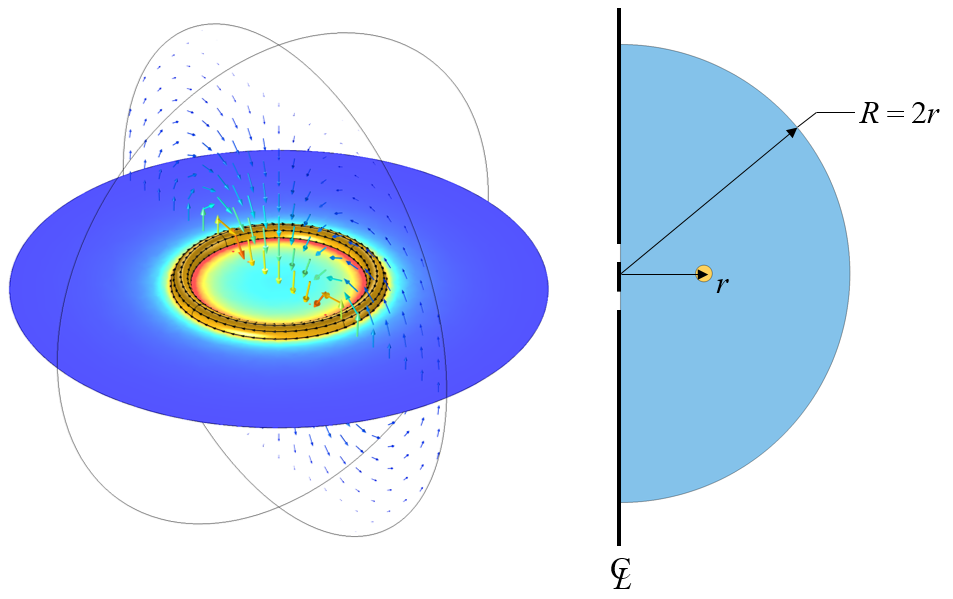
A circular coil in a spherical modeling domain can be modeled via a 2D axisymmetric model. The domain radius is normalized with respect to the coil radius.
We will consider two different boundary conditions along the outside radius of the modeling domain shown above: the Magnetic Insulation (MI) boundary condition and the Perfect Magnetic Conductor (PMC) boundary condition. The Magnetic Insulation condition can be physically interpreted as a boundary to a domain that has infinite electrical conductivity. That is, the Magnetic Insulation condition implies that our coil is enclosed within a sphere of very high conductivity. Currents can flow and be induced on a magnetic insulation boundary. Mathematically speaking, the magnetic insulation fixes the field variable that is being solved for to be zero at the boundary; it is a homogeneous Dirichlet boundary condition.
On the other hand, the Perfect Magnetic Conductor boundary condition can be thought of as the opposite boundary condition. Mathematically, it enforces the homogeneous Neumann condition, meaning the derivative of the solution field in the direction normal to the boundary is zero. No current can flow, nor be induced on, a perfect magnetic conductor boundary.
Since these two boundary conditions can be thought of as opposites, let’s take a look at what happens to the solution as we solve the above problem with an increasing radius of the surrounding air sphere and monitor the computed coil inductance. We can perform a parametric sweep over the domain radius and then take the average of the solutions for the two different boundary conditions by joining solutions. These results are shown in the plot below, and we can observe that the solution for the inductance converges with increasing domain radius. We can also observe that the average of the two solutions converges even faster.
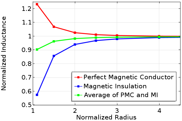
Normalized inductance of a coil with an increasing radius for different boundary conditions.
From the above plot, we can conclude that it doesn’t matter which boundary condition we use for this axisymmetric problem, as long as we study the solution with an increasing domain radius. We can also conclude that we can run the model with a relatively smaller domain radius and with both Magnetic Insulation and Perfect Magnetic Conductor boundary conditions to take the average of the two cases. This average, even for a small radius, will give a good prediction of the solution at larger domain radii.
Replacing Boundary Conditions with Domain Conditions
We can, in fact, avoid the question of boundary conditions entirely by truncating our modeling domain with a domain condition known as an infinite element domain. The infinite element domain requires that you add an additional domain as a layer around the exterior of the modeling domain. The software then internally performs a coordinate stretching within this domain such that the domain is infinitely large, for all practical purposes. Thus, the solution from a model with infinite element domains will be the same as when the domain radius is increased.
The advantage of the infinite element domain is that it obviates the question of choosing between boundary conditions as well as the question of the domain size. The infinite element domain can be placed in very close proximity to the coil — it could even be touching. The only additional work that the infinite element introduces is in the model and the meshing setup. Also, the solution time and memory requirements for larger 3D models can be greater. These are, however, only very small prices to pay for the added convenience.
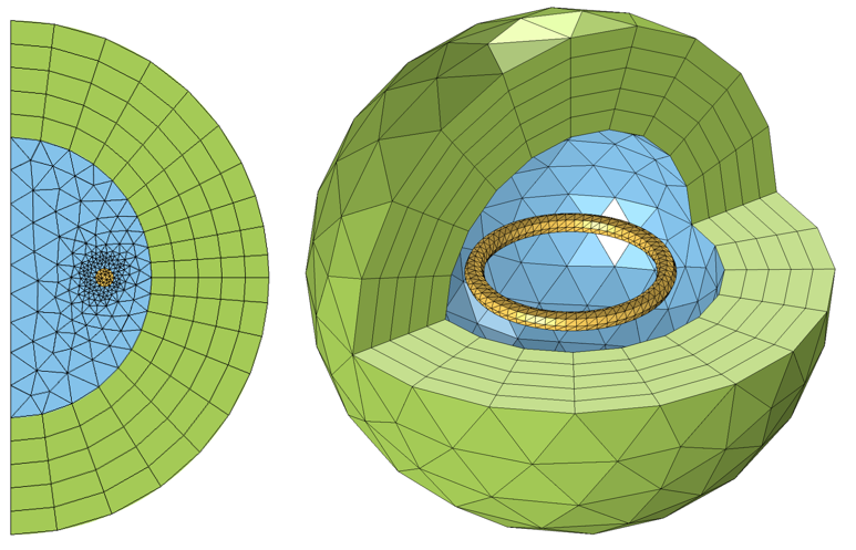
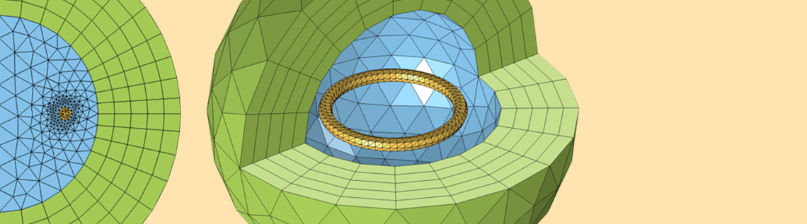
The meshes for typical 2D axisymmetric and 3D infinite element domains.
Closing Remarks on Choosing Boundary Conditions for Coil Modeling
We have looked at three different approaches for truncating a domain when modeling an electromagnetic coil in free space: the Magnetic Insulation boundary condition, the Perfect Magnetic Conductor boundary condition, and the infinite element domain. When using the Magnetic Insulation and Perfect Magnetic Conductor boundary conditions, you must study model convergence with an increasing domain radius, and as the domain radius increases, the solutions will all converge toward the same value. Taking the average of the two cases can predict what will happen at larger domain radii. You can also put in a little bit more effort and use the infinite element domains to get to the same answer.
Also keep in mind that, if your coil extends to the boundaries of the modeling domain, you need to provide a current return path via the Magnetic Insulation boundary condition. If there are domain boundaries that represent a metallic enclosure and if you are modeling in the frequency domain, then also look toward the Impedance boundary condition, which is useful for modeling lossy materials such as metals.
If you have a model with symmetry, you can also use the Magnetic Insulation and Perfect Magnetic Conductor boundary conditions to enforce different kinds of symmetry, as explained in our earlier blog post on exploiting symmetry to simplify magnetic field modeling.
Further Resources
If you are just getting started with coil modeling in the AC/DC Module in COMSOL Multiphysics, you should also take a look at the following example models:
- Modeling of a 3D Inductor
- Inductance of a Power Inductor
- Magnetic Field of a Helmholtz Coil
- Multi-Turn Coil Above an Asymmetric Conductor Plate
- Multi-Turn Coil Winding around a Ferromagnet
- Mutual Inductance and Induced Currents Between Single-Turn Coils
- Mutual Inductance and Induced Currents in a Coil Group
- Mutual Inductance and Induced Currents in a Multi-Turn Coil
- Modeling a Spiral Inductor Coil
- Integrated Square-Shaped Spiral Inductor
What kind of coil modeling would you like to do with COMSOL Multiphysics and the AC/DC Module? Contact us and let us know.

Comments (0)