

We have all experienced the boredom and frustration of being stuck in a traffic jam. Very often, traffic congestion comes and goes for no obvious reason. Employing the analogy to gas dynamics, we can now simulate traffic flow using the equation-based modeling capabilities of COMSOL Multiphysics and gain a better understanding of why congestion happens.
More Cars than Roads
The Texas Transportation Institute estimates that in 2000, the 75 largest metropolitan areas experienced 3.6 billion vehicle hours of delay, resulting in 5.7 billion gallons in wasted fuel and $67.5 billion in lost productivity. We are inclined to blame bad weather, poorly timed traffic lights, and other drivers for not merging into the exit lane in advance. It must be someone’s fault.
According to a 2005 report by the Federal Highway Administration (FHA), about 40% of traffic congestion in the U.S. occurs as a result of sheer volume of traffic. Between 1980 and 1999, vehicle miles of travel grew by 76% while the amount of new roads or lanes increased only by 1.5%. There simply aren’t enough or large enough roads. However, can a large volume of vehicles alone cause congestion? If everyone drives at a constant speed of 55 mph, a congestion is unlikely to happen, isn’t it?
Phantom of the Road
A group of Japanese scientists, Sugiyama et al., conducted an experiment in March 2008 to prove us wrong. As shown in this video, 22 homogeneously distributed cars are initially traveling at the same speed on a circuit. A traffic jam then appears out of nowhere and propagates backward like a solitary wave.
MIT professor Rodolfo Rosales calls this phenomenon phantom traffic jam, which arises without any bottleneck or obstacle. When the traffic density passes a critical threshold, even a small perturbation in the traffic flow can amplify into traveling waves of high traffic density. This means that in rush hour traffic, when we reach for a cup of coffee or fiddle with the radio, the perturbation in vehicle speed might just be enough to leave the road haunted by phantom traffic jams.
Modeling Traffic Congestion in COMSOL Multiphysics
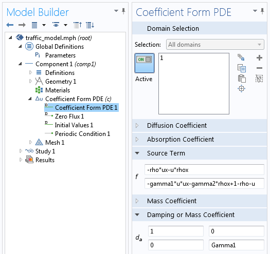
Besides experiments, phantom traffic jams can be observed in a numerical simulation study. Since traffic flow resembles inviscid fluid flow, the phantom traffic jams can be modeled as detonation waves produced by explosions. A widely known model depicting this phenomenon is the Payne-Whitham model. The corresponding partial differential equations (PDEs) are implemented as an equation-based model in COMSOL Multiphysics.
The equations for the density and velocity of the cars are implemented directly in the COMSOL Multiphysics user interface (UI). Because it does not require any coding, such a model can be implemented in a few minutes.
The COMSOL Multiphysics model consists of a one-dimensional line 500 meters in length with periodic boundaries. In the following animation, the two ends of the line are connected to form a circuit, where 27 cars are traveling clockwise. Traffic density is represented by the radius of the red curve on the outside as well as the colors on the inner ring. A small initial perturbation is introduced to the traffic flow, which later grows into a traveling peak on the traffic density curve. Correspondingly, the congestion locations change from green to yellow and red in the color ring. We can clearly see how small sections of congestion emerge, form a single traffic jam, and propagate backwards in traffic, i.e. counter-clockwise, just like in the video of the experiment we linked to above.
Traffic density evolution normalized against maximum density.
Reducing the number of cars on the circuit can obviously alleviate the congestion. Another interesting aspect of the model is that we assume each driver has a reaction time of 3.3 seconds. That means a driver needs 3.3 seconds to fully adjust their speed to match the speed of traffic. This delay in reaction is partially responsible for amplifying the initial perturbation. Supposing all the cars are equipped with radar-guided cruise control and the reaction time is reduced to 0.4 seconds, the congestion can be eliminated altogether — something to factor in next time you buy a car!
Learn More About Equation-Based Modeling
Although the Payne-Whitham model only simulates a simplified version of our daily commute, more complexity can be added using the COMSOL Multiphysics equation-based modeling capabilities. The COMSOL software can not only handle different types of PDEs, but also ordinary differential equations (ODEs), algebraic equations, and transcendental equations. These capabilities are all included in the core functionality of COMSOL Multiphysics.
Additional Resources
- To benefit more from the flexibility of building your own custom models, be sure to check out the following:
- U.S. Department of Transportation, Federal Highway Administration. Office of Operations. 21st century operations using 21st century technologies.
- Y. Sugiyama et al. “Traffic jams without bottlenecks—experimental evidence for the physical mechanism of the formation of a jam.“
- R. Rosales et al. “Traffic modeling – phantom traffic jams and traveling jamitons.“
- M. Flynn et al. “Self-sustained nonlinear waves in traffic flow.“

Comments (1)
Sam Young
December 20, 2018Great article! Is it possible for you to post the simulation file? I’m interested in investigating this more.