

When you think of evaporation, you probably think of the cup on your desk that spreads the aroma of coffee or tea. But evaporation is also a process with many industrial and scientific applications, ranging from meteorology to food processing. Here, we give an introduction to modeling evaporative cooling using a cup of coffee as an example.
Editor’s note: The original version of this post was published on December 8, 2014. It has since been updated to reflect new features and functionality available in the Heat Transfer Module.
Some Basic Concepts of Modeling Evaporation in COMSOL Multiphysics
Evaporation is a process that occurs if some substance in its liquid phase vaporizes into a gas mixture that is not saturated with the substance. We exemplify this process and its characteristic properties by using water as the liquid substance and air as the gas.
Let’s first define the saturation pressure, p_{sat}, at which the gas phase of a substance is at equilibrium with its liquid phase. It is strongly temperature dependent and there are many approximations out there, which are all very similar but not exactly the same.
The COMSOL Multiphysics® software uses the following approximation from Principles of environmental physics by J. L. Monteith and M. H. Unsworth (1990):
(1)
For ideal gases, it is easy to determine the saturation concentration at which the relative humidity is 100% with:
(2)
where R is the ideal gas constant.
The thermodynamic properties of moist air depend on the fraction of water vapor. A mixture formula is used to describe the properties with the proportional amount of dry air and water vapor. Assuming air behaves as an ideal gas, the density reads:
(3)
More details and references about the implementation of the moist air properties as used by COMSOL Multiphysics can be found in the Heat Transfer User’s Guide (located within the Heat Transfer Module).
Modeling Evaporative Cooling: A Coffee Cup Example
Before setting up the COMSOL Multiphysics model, let’s consider the effects causing the cooling of the coffee as it evaporates.
We assume a slight air draft around the cup (or beaker, since there is no handle in this case) that accelerates the cooling by transporting heat and removing water vapor from the surface. At the coffee–air interface, vapor escapes from the liquid into the air, causing additional cooling by evaporation.
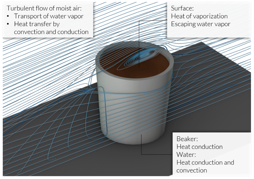
Sketch of the participating effects in a coffee cup.
How to Implement the Evaporative Cooling Effect in a Model
The first step is to make use of the symmetry, which reduces the model size and thereby the computational time. For the slight air draft, we use the Turbulent Flow interface with a constant air velocity. A reasonable approximation here is to assume that the flow field won’t change with a change in temperature and moisture content. Hence, we calculate a stationary velocity field in an initial study.
What else do we need to model the evaporative cooling effect?
Thanks to the predefined Heat and Moisture multiphysics coupling, it is easy to implement the evaporative cooling effect in a COMSOL Multiphysics model.

Multiphysics interfaces for modeling heat and moisture transport in different media.
The Moist Air multiphysics interface automatically couples the Heat Transfer in Moist Air interface with the Moisture Transport in Air interface and thus describes the heat and moisture transport as well as the interaction of both processes using the Heat and Moisture multiphysics coupling node. To also couple the flow field to both of the transport interfaces, add the Nonisothermal Flow and Moisture Flow multiphysics coupling nodes. Alternatively, the Heat and Moisture Flow interface is available, which already provides all required interfaces and their couplings.
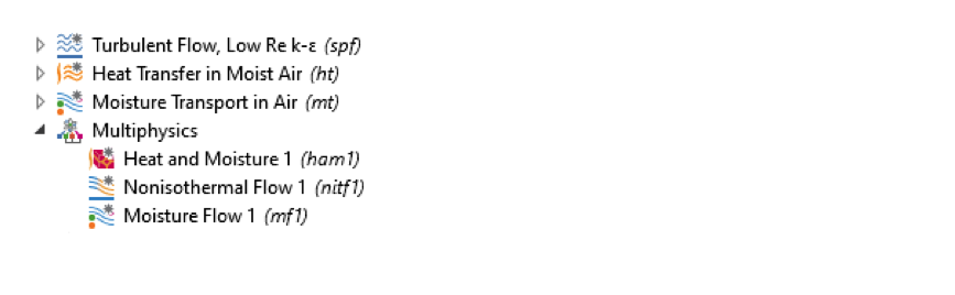
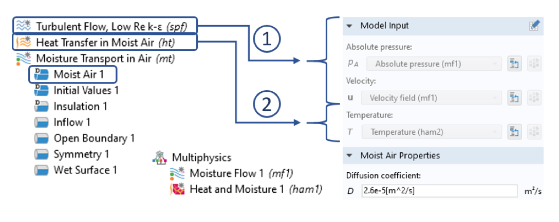
Required interfaces and multiphysics nodes for coupling turbulent flow and heat and moisture transport.
The Nonisothermal Flow node defines the coupling between the flow and the heat interfaces. Note that in this case, we do not need the strongly coupled approach, since the flow field is assumed to be independent of the temperature or moisture content. In other words, the material properties are assumed to be constant for the calculation of the flow. The Boussinesq approximation can be used for this purpose. The Nonisothermal Flow node also accounts for the turbulence effects in the heat transfer interfaces. The Moisture Flow node couples the flow and the moisture transport interfaces, and turbulence effects are taken into account in the transport interface.
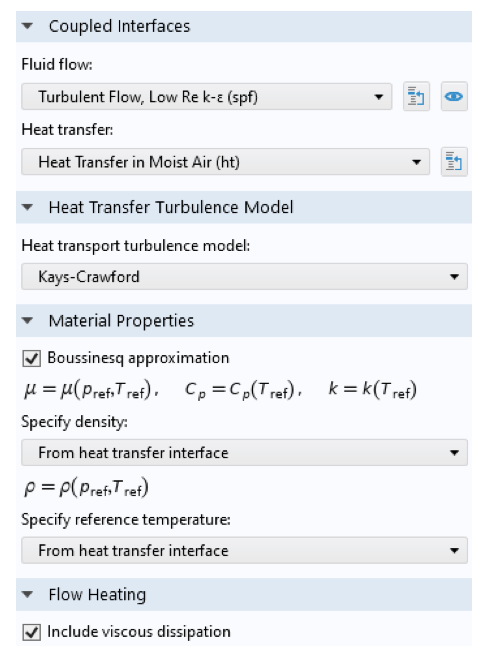
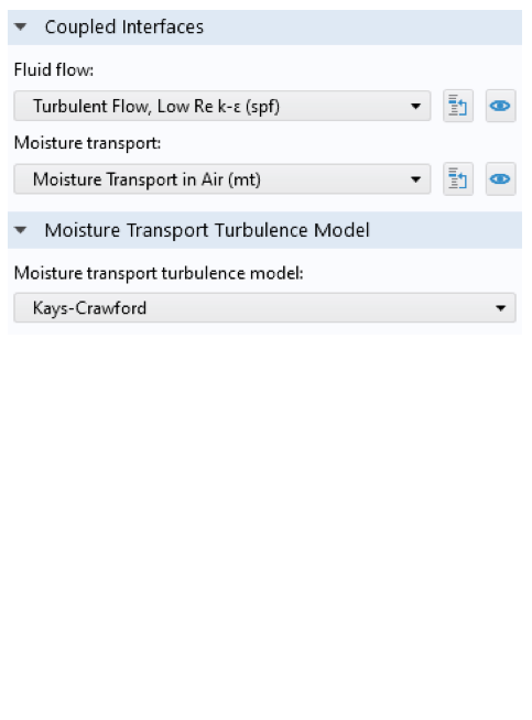
Multiphysics nodes for the nonisothermal flow (left) and moisture flow (right). The Nonisothermal Flow node settings define the nonisothermal flow properties: the names of the interfaces, a turbulence model for heat, common material properties for the heat transfer and flow interface, and flow heating. The Moisture Flow node settings define the names of the interfaces and a turbulence model for moisture transport.
The Heat Transport interface calculates the temperature distribution in moist air, and this requires the relative humidity calculated with the Moisture Transport interface. The relative humidity in turn depends on the temperature. At the wet water surface, the relative humidity will always be 100%. Hence, the saturation concentration c_\textrm{sat} is reached, and is defined according to Equation 2.
The Wet Surface boundary condition is used to compute the evaporation flux g_\textrm{evap} from the surface to the moist air. If the Include latent heat source on surfaces check box is selected (default), the latent heat flux is computed according to Q_\textrm{evap}=-L_\textrm{v}g_\textrm{evap} with the temperature-dependent latent heat of water L_\textrm{v}. All in all, it is a strongly coupled phenomena that is implemented in no time with the available interfaces and couplings.
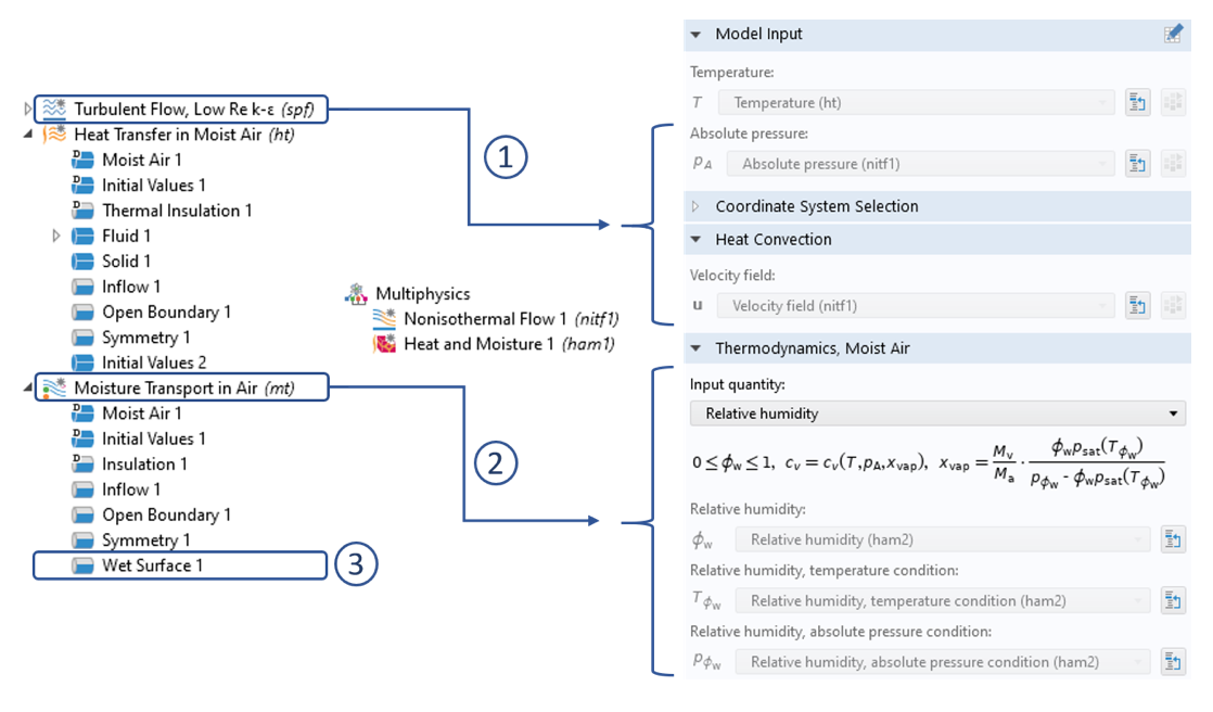
Settings for heat transfer inside the moist air domain: (1) Coupling of the flow field via the Nonisothermal Flow multiphysics node for convective transport of the moist air. (2) Coupling to the Moisture Transport in Air interface via the Heat and Moisture multiphysics node, which gives us the correct input of relative humidity to determine the moist air properties according to Equation 2. (3) The Wet Surface interface calculates the evaporative flux from this surface. If the Include latent heat source on surfaces check box within the Heat and Moisture multiphysics node is enabled, the cooling due to evaporation is taken into account.
Settings for the moisture transport inside the moist air domain: (1) Coupling of the flow field via the Moisture Flow multiphysics node for convective transport of water vapor. (2) Coupling to the Heat Transfer in Moist Air interface via the Heat and Moisture multiphysics coupling node, which ensures the correct computation of relative humidity.
Next, we take a look at the results of a time-dependent study over 20 minutes. The initial coffee temperature was 80°C, and air at 20°C enters the modeling domain with a relative humidity of 20% causing the cooling. Below, you can see the resulting temperature and relative humidity distribution, both after 20 minutes.


Temperature distribution (left) and relative humidity (right) after 20 minutes.
Does evaporation have a strong influence on the cooling? We can find out by comparing the average temperature of the coffee — including evaporation — to that of the same model neglecting evaporation.
To do so, we’ll set up a third study solving for the Heat Transfer in Moist Air and Moisture Transport in Air interfaces and disable the Heat and Moisture multiphysics node. The resulting plot clearly shows that cooling due to evaporation has a significant impact on the overall cooling:
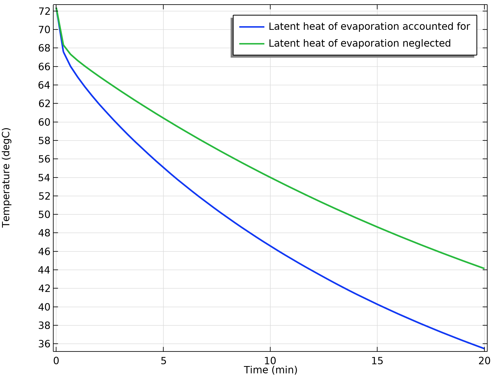
Comparison of the average coffee temperature over time.
Next Step
This blog post has shown the basic aspects you need to consider when modeling evaporative cooling. Explore the model discussed here by downloading the documentation and MPH-file from the Application Gallery.


Comments (24)
Morteza Alipanah
October 31, 2016Hi,
The way of how to simulate the evaporating water is explained here. can you please let me know how can we simulate the condensing water vapor mixed in the moist air into a liquid.
Thanks
Nancy Bannach
November 4, 2016Dear Morteza,
the way of modeling condensation is exactly the same. If condensation or evaporation occurs depends on the temperature. This determines the saturation pressure/concentration and hence the heat source/sink term. Just set the relative humidity at the air inlet to 1 and set a higher ambient temperature and lower water temperature.
In this example we neglected the decreasing of the water level in the beaker due to the relatively small amount of water evaporating into the air. If you want to include such effects (also rising due to condensation) you can add a deformed mesh physics interface to track the water level according to the amount of water entering. This adds more complexity and numerical effort to your model. You can have a look at the following example of freeze drying:
https://www.comsol.de/model/freeze-drying-3924
If you need further assistance feel free to contact our support team https://www.comsol.de/support.
Have a nice day,
Nancy
Yousra Toulan
August 9, 2023Hi,
Please, Could you tell me how can I calculate the amount of condensed water?
Omar Al-Rawi
February 6, 2017Hi,
Many thanks for this intensive explaination.
You have used the Lagrange multiplier expression, c_lm, to represent the flux from the water surface. Does this expression include the convection flow effect in air in addition to the diffusive effect and can I check that? Also, why this expression gives results lower than if I define the flux as:
Flux = -D*concentration gradient
Thanks
Nancy Bannach
February 7, 2017Dear Omar,
this is a kind of numerical question. I’m not a mathematician, so I explain it with my own words. At the surface you have a fixed concentration (Dirichlet boundary condition). In the equation COMSOL solves (weak form), the Dirichlet boundary condition vanishes, but c=c0 holds of course.
Now, you only know the concentration at the boundary, but not the flux. So using the concentration gardient is more an approximate flux since you calculate this gradient with the solution for c inside the domain.
With the Lagrange multiplier you add additional equations for the flux on this boundary, which answer the question which flux must be applied to get the concentration c=c0. And then c_lm gives the exact flux. Often this difference is small, but especially in multiphysics problems you should use this approach. Some interfaces have this active by default. This is the “Compute boundary fluxes” check box in the Interface settings “Discretization” section.
The variable c_lm is the total flux. But since the velocity is zero at the ware surface (no-slip) wall boundary condition the flux is by diffusion. Of course, the convection in the air affects this flux, because heat and concentration is carried away and this affects the saturation concentration.
I hope this answers your question.
Have a nice day,
Nancy
Omar Al-Rawi
February 24, 2017Hi Nancy,
Many thanks for this explaination.
Indeed, I have another question. Based on the Reynolds number you’ve mentioned (1500), which I don’t know how is calculated, the flow should be laminar. So, why did you impose the model with turbulent flow?
My wondering is becuase that I’m modelling evaporation of two neighbouring droplets under forced convective environment inside a duct with size (W20, H10 and D20mm). I’ve imposed the air flow is modeled with laminar flow, and the air flow velocities are (0.02, 0.2 and 2m/s). Just with the last air flow velocity, the model doesn’t work although the flow is still with laminar regime. Therefore, I am asking that becuase that I have to change the flow regime from laminar to turbulent with low Re number.
Regards,
Omar
Nancy Bannach
February 24, 2017Hi Omar,
unfortunately there is not one single critical Reynoldsnumber where flow turns from laminar into turbulent. The critical Reynoldsnumber strongly depends on the geometry. If you would remove the cup from the flow domain, then it could be laminar. But if you place an obstacle in a flow stream, you almost always introduce turbulence.
The calculation of the Reynoldnumber uses a characteristic length. For a pipe, this is the radius or diameter and it is just a convention what you use. Hence, the value for the critical Reynolds number changes.
Maybe another blog post is interesting for you (coincidentally I was the autor again 😉 ):
https://www.comsol.com/blogs/characterizing-flow-choosing-right-interface/
In general fluid flow is a very challenging topic and still a huge topic in numerics. For your specific problem I recommend to use our Support Center or Discussion Forum, which is dedicated to talk about individual tasks.
Have a nice day,
Nancy
Israr Ahmad
April 3, 2017Hi Ma’am
I have been working on electronic cooling by electrowetting on dielectric (EWOD) technique. where droplet is manipulated through sequential actuation voltage over the electrode. However, the droplet is transported over the hot spot where constant heat flux has been provided. The droplet is supposed to carry the heat via conduction, convection and phase change and moved over another electrode. Till now, i have been able to solve single phase cooling process with laminar two phase flow phase field and heat transfer in fluid module but facing difficulty to model evaporative cooling.
In this example, the draft of air itself over the surface transported the heat and vapor into it. But in my case, there is still air in between two plates. Can you please give me idea for modelling evaporative cooling in my model.
With Regards
Bridget Cunningham
April 3, 2017Hello Israr,
Thank you for your comment.
For questions related to your modeling, please contact our support team.
Online support center: https://www.comsol.com/support
Email: support@comsol.com
Best,
Bridget
Victor Casquero Pretell
April 28, 2017Hi Nancy,
The K value for the transport of heat in the evaporation of water, was assumed value 100 or it can be estimated mathematically.
Nancy Bannach
May 2, 2017Dear Victor,
I assume your question about K relates to the 5.3 version of the model using the Moisture Transport in Air interface. The approach discussed here is a little different.
You can find an explanation about K in the related pdf document:
“The evaporation rate must be chosen so that the solution is not affected if further
increased. This corresponds to assuming that vapor is in equilibrium with the liquid.”
If this does not answer your question, contact our support team for detailed discussions (support@comsol.com).
Best regards,
Nancy
Omar Al-Rawi
June 12, 2017Hi again Nancy,
My question may not relate to this blog but hopefully you can help me.
If I want to send your model, which involves three studies, to HPC, which command I can use into the shell file to run all these studies?
Actually, I have used this command to run one study so will it be different in the case of your model?
“comsol batch -np $NSLOTS -tmpdir $TMPDIR -inputfile input_model.mph -outputfile output_model.mph”
Regards,
Omar
Bridget Cunningham
June 12, 2017Hello Omar,
Thanks for your comment.
In regards to this question, please contact our Support team.
Online Support Center: https://www.comsol.com/support
Email: support@comsol.com
Omar Al-Rawi
August 29, 2017Dear All,
I have other questions about this model, particularly the heat transfer interface.
1- In the hea tansfer in fluid 1 subnode, the “Equivalent conductivity for convection” feature is activated, and I think is because the convection inside water is neglected. But the question is that base on what the temperature difference is defined as 3[K], and what does this parameter mean?
2- In the heat transfer in fluid 1, 2 and solid, why did you select the temperature in the “Model input” related to the “ht” interface instead “nitf1” multiphysics node?
Regards,
Omar
elias Yazdanshenas
September 19, 2017Dear all,
I am looking for how to change the fluid phase in the condenser by losing heat. Please let me know if you have any idea about that.
Regards,
Elias
Nancy Bannach
September 20, 2017Dear Omar,
I’m not sure to which version of the model you refer. If I open the model from the gallery the Temperature difference for Equivalent conductivity is set to “Automatic”. Otherwise a user-defined temperature difference can be a guess or maybe estimated from similar problems. The temperature difference determines the Rayleigh number which again is used to estimate the convective heat flux by Nusselt number correlations (check the manual for more details).
About your second question (I refer to the version 5.3 model from the gallery):
The temperature from nitf is not available for solids and fluid1, because there we don’t solve for Nonisothermal flow. Otherwise, in most cases the temperatures from nitf and ht are the same and you can rely on the automatic seetings.
There could be a difference depending on how you build your model and studies. If you are unsure, you can plot nitf.T-ht.T. This should be zero.
Dear Elias,
I’m not sure if I understand your question. In general, if evaporation/condensation occurs depends on the temperatures and is calculated automatically. If you look for other phase changes, then the “Phase Change Material” feature could be interesting.
But I recommend to contact our support team for a detailed discussion
Online Support Center: https://www.comsol.com/support
Email: support@comsol.com
Best regards,
Nancy
Steven Spielman
January 3, 2018Does the “evaporation rate” parameter have any physical significance? Why does it have the name it does, rather than, say, “Mangione coefficient” or “turbo encabulator”. I’m serious. The documentation I’ve seen would make exactly as much sense, had the name been replaced with either of these options.
Nancy Bannach
January 4, 2018Dear Steven,
“Evaporation rate” is a common name that is used to describe drying processes and many other processes that deal with evaporation, e.g. food processes.
The evaporation rate is a property that depends on the material properties and the process itself.
However, in this case it is just chosen to be large enough such that the approach is valid. This doesn’t mean that it has no physical meaning but the exact value doesn’t play a role for the physics described here as long as it is large enough.
See also:
https://www.comsol.de/model/evaporation-in-porous-media-with-small-evaporation-rate-21931
Have a nice day,
Nancy
saiedeh Arabi
February 9, 2018Dear all,
I am looking for how to change the fluid phase (liquid water to steam) by earning the heat source. Please let me know if you have any information.
Caty Fairclough
February 12, 2018Hi Saiedeh,
Thanks for your comment.
For your question, please contact our Support team.
Online Support Center: https://www.comsol.com/support
Email: support@comsol.com
Mostafa Abdelrehim
November 1, 2018Hi Nancy
Thanks for that tutorial,
I have a simple question, why you did not use the “Heat Transfer with Phase Change” interface to model the evaporization of water? I was expecting that when I start reading but you end up using different physics.
actually my problem that I am currently working on is similar, I have a liquid that passing through some channel that have heat source on one of its walls , and due to that heat some of the liquid will evaporate to a gaseous phase in a phase change manner. I am expecting that walls will be cooled due to the latent heat absorbed by the liquid to be trasfered to vapor. Thanks
Nancy Bannach
November 7, 2018Hi Mostafa,
let’s take water as an example. When water freezes or ice melts you have one material in different physical states (liquid or solid).
When water evaporates you have one liquid phase that evaporates into an existing gaseous phase (air). So you have two materials (water+air) and the phase change takes place at the interface between these materials.
The Heat Transfer with Phase Change is not really suitable for that.
The approach that is used in this blog post should work for your problem as well. Since this blog post relates to an older version, you may want to have a look at this blog post:
https://www.comsol.de/blogs/how-to-model-moisture-flow-in-comsol-multiphysics/
The principle is the same, but it shows the new interfaces and multiphysics couplings that are available now.
Best regards,
Nancy
Yousra Toulan
August 9, 2023Dear Dr. Nancy,
I want to simulate solar still which is based on evaporation and condensation, I didn’t find videos or files that explain that. Could you tell me about videos or documents that explain that?
Thanks in advance.
Quadri Adebayo
March 31, 2024Hello,
I’m trying to run the same analysis but the geometric of the cup is different, I getting errors during the computation of the TURBULENT FLOW, LOW RE K- ε (SPF) physics leading to my inability to continue the analysis. Can I get help?