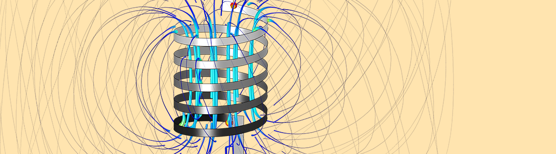

If you design electromagnetic coils, the combination of the AC/DC and Optimization modules with the COMSOL Multiphysics® software gives you the power to quickly come up with improved design iterations. Today, we will look at designing a coil system to achieve a desired magnetic field distribution by changing the coil’s driving currents. We will also introduce three different optimization objectives and constraints. This topic is of interest to anyone who is modeling coils or curious about optimization.
The Magnetic Field Model and Optimization Problem Statement
The problem we will look at today is the optimization of a ten-turn axisymmetric coil structure, as shown in the image below. Each of the five turns on either side of the xy-plane is symmetrically but independently driven.
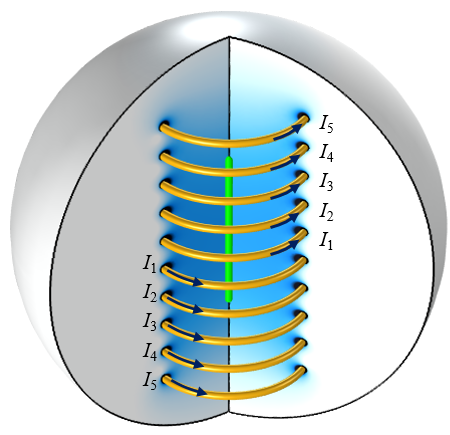
A ten-turn coil with five independently driven coil pairs. The objective is to alter the magnetic field at the centerline (green highlight).
The coil is both rotationally symmetric and symmetric about the z = 0 plane, so we can reduce the computational model to a 2D axisymmetric model, as shown in the schematic below. Our modeling domain is truncated with an infinite element domain. We use the Perfect Magnetic Conductor boundary condition to exploit symmetry about the z = 0 plane. Thus, our model reduces to a quarter-circle domain with five independent coils that are modeled using the Coil Domain feature.
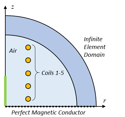
A schematic of the computational model.
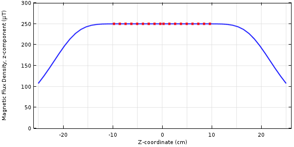
If all of the coils are driven with the same current of 10 A, we can plot the z-component of the magnetic flux density along the centerline, as shown in the image below. It is this field distribution along a part of the centerline that we want to change via optimization.

The magnetic field distribution along the coil centerline. We want to adjust the magnetic field within the optimization zone.
From the image above, we see the magnetic field along a portion of the centerline due to a current of 10 A through each coil. It is this field distribution that we want to change by adjusting the current flowing through the coils. Our design variables are the five unique coil currents: I_1, I_2, \dotso, I_5. These design variables have bounds: -I_{max}\le I_{1,\dotso,5}\le I_{max}. That is, the current cannot be too great in magnitude, otherwise the coils will overheat.
We will look at three different optimization problem statements:
- To have the magnetic field at the centerline be as close to a desired target value as possible
- To minimize the power needed to drive the coil, along with a constraint on the field minimum at several points
- To minimize the gradient of the magnetic field along the centerline, along with a constraint on the field at one point
Optimizing for a Particular Field Value
Let’s state these optimization problems a bit more formally. The first optimization problem can be written as:
& \underset{I_1, \ldots ,I_5}{\text{minimize:}}
& & \frac{1}{L_0} \int_0^{L_0} \left( \frac{B_z}{B_0} -1 \right) ^2 d l \\
& \text{subject to:}
& & -I_{max} \leq I_1, \ldots ,I_5 \leq I_{max}\\
\end{aligned}
The objective here is to minimize the difference between the computed Bz-field and the desired field, B0 = 250μT, integrated over a line along the center of the coil, stretching from z = 0 to z = L0. Note that this objective is normalized with respect to L0 and B0. This is done such that the magnitude of this objective function will be around one. The scaling of the objective function should always be done for any optimization problem.
Now, let’s look at the implementation of this problem within COMSOL Multiphysics. We begin by adding an Optimization interface to our model, which contains two features. The first feature is the Global Control Variables, as shown in the screenshot below. We can see that five control variables are set up: I1,...,I5. These variables are used to specify the current flowing through the five Coil features in the Magnetic Fields interface.
The Initial Value, Upper Bound, and Lower Bound to these variables are also specified by two Global Parameters, I_init and I_max. Also note that the Scale factor is set such that the optimization variables also have a magnitude close to one. We will use this same setup for the control variables in all three examples.
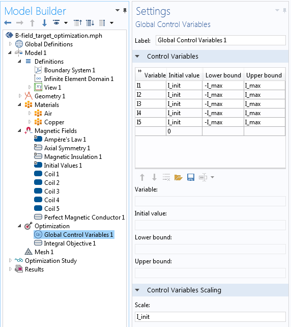
Setting up the Global Control Variables feature, which specifies the coil currents.
Next, the objective function is defined via the Integral Objective feature over a boundary, as shown in the screenshot below. Note that the Multiply by 2πr option is toggled off.
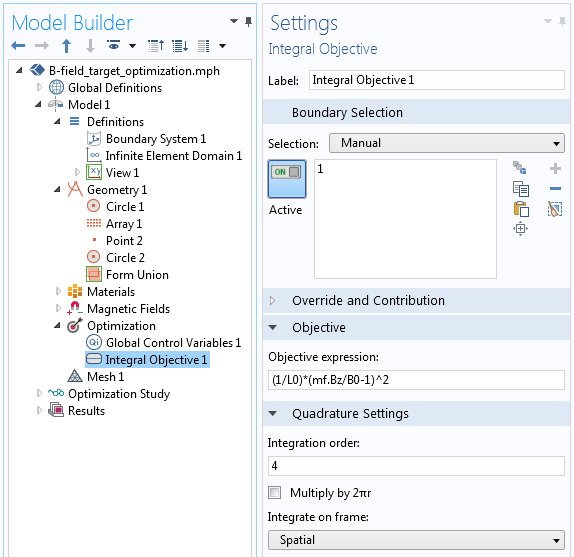
The implementation of the objective function to achieve a desired field along one boundary.
We include an Optimization step in the Study, as shown in the screenshot below. Since our objective function can be analytically differentiated with respect to the design variables, we can use the SNOPT solver. This solver takes advantage of the analytically computed gradient and solves the optimization problem in a few seconds. All of the other solver settings can be left at their defaults.
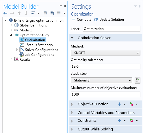
The Optimization study step.
After solving, we can plot the fields and results. The figure below shows that the Bz-field matches the target value very well.
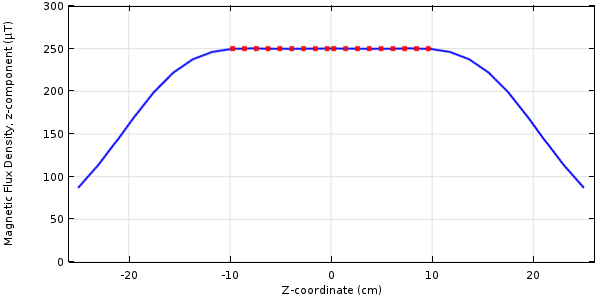
Results of optimizing for a target value of magnetic flux along the centerline.
Minimizing the Power with a Constraint on the Field
Our second optimization problem is to minimize the total power needed to drive the coil and to include a constraint on the field minimum at several points along the centerline. This can be expressed as:
& \underset{I_1, \ldots ,I_5}{\text{minimize:}}
& & \frac{1}{P_o}\sum_{k=1}^{5} P_{coil}^k \\
& \text{subject to:}
& & -I_{max} \leq I_1, \ldots ,I_5 \leq I_{max}\\
& & & 1 \le B_z^i/B_{0}, i=1, \ldots, M
\end{aligned}
where Po is the initial total power dissipated in all coils and P_{coil}^k is the power dissipated in the kth coil.
We further want to constrain the fields at M number of points on the centerline to be above a value of B0.
The implementation of this problem uses the same Global Control Variables feature as before. The objective of minimizing the total dissipated coil power is implemented via the Global Objective feature, as shown in the screenshot below. The built-in variables for the dissipated power (mf.PCoil_1,...,mf.PCoil5) in each Coil feature can be used directly. The objective is normalized with respect to the initial total power so that it is close to unity.
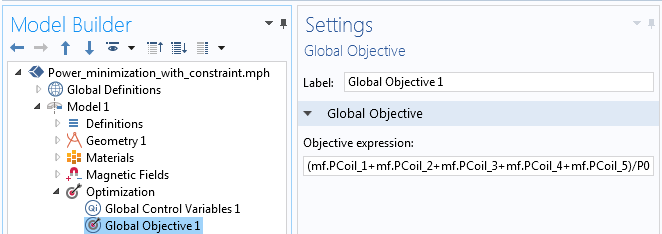
Implementation of the objective to minimize total power.
The constraint on the field minimum has to be implemented at a set of discrete points within the model. In this case, we introduce five points evenly distributed over the optimization zone. Each of these constraints has to be introduced with a separate Point Sum Inequality Constraint feature, as shown below. We again apply a normalization such that this constraint has a magnitude of one. Note that the Multiply by 2πr option is toggled off, since these points lie on the centerline.
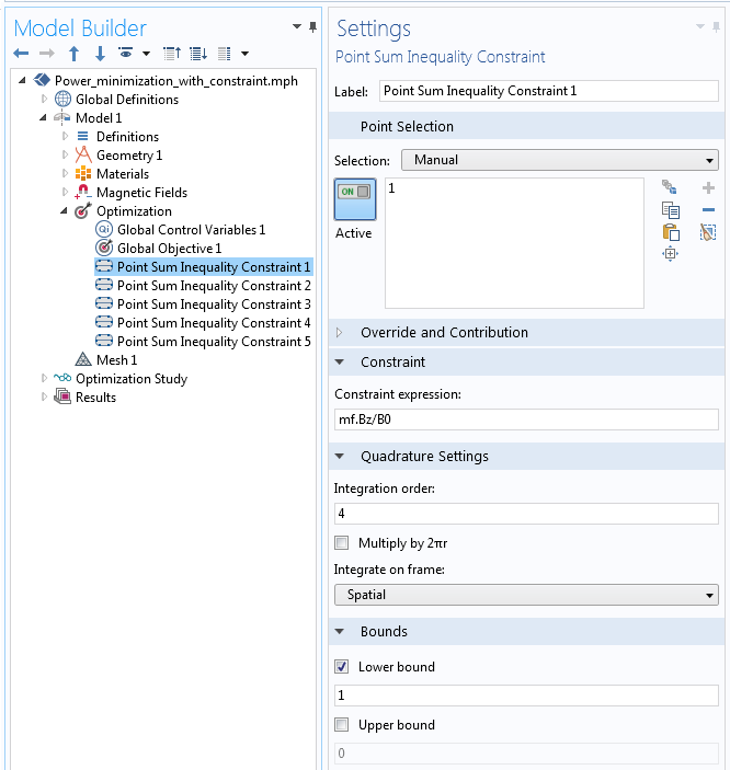
The implementation of the constraint on the field minimum at a point.
We can solve this problem using the same approach as before. The results are plotted below. It is interesting to note that the minimal dissipated power solution does not result in a very uniform field distribution over the target zone.
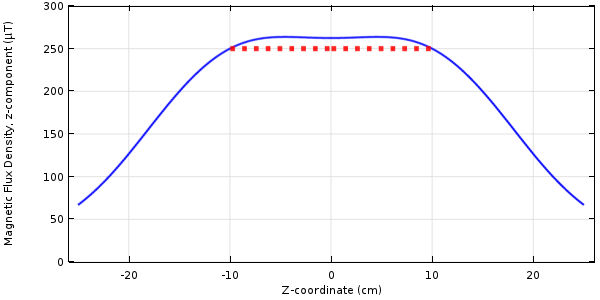
Results of optimizing for a minimum power dissipation with a constraint on the field minimum.
Minimizing the Gradient with a Constraint on the Field
Finally, let’s consider minimizing the gradient of the field along the optimization zone, with a constraint on the field at the centerpoint. This can be expressed as:
& \underset{I_1, \ldots ,I_5}{\text{minimize:}}
& & \frac{1}{L_0 B_{0}} \int_0^{L_0} \left( \frac{\partial B_z}{\partial z } \right) ^2 d l \\
& \text{subject to:}
& & -I_{max} \leq I_1, \ldots ,I_5 \leq I_{max}\\
& & & B_z(r=0,z=0) = B_0 \end{aligned}
The constraint here fixes the field at the centerpoint of the coil. Although the Optimization interface does have an explicit equality constraint, we can achieve the same results with an inequality constraint with equal upper and lower bounds. We again apply a normalization such that our constraint is actually 1 \le B_z/B_0 \le 1, as shown in the image below.
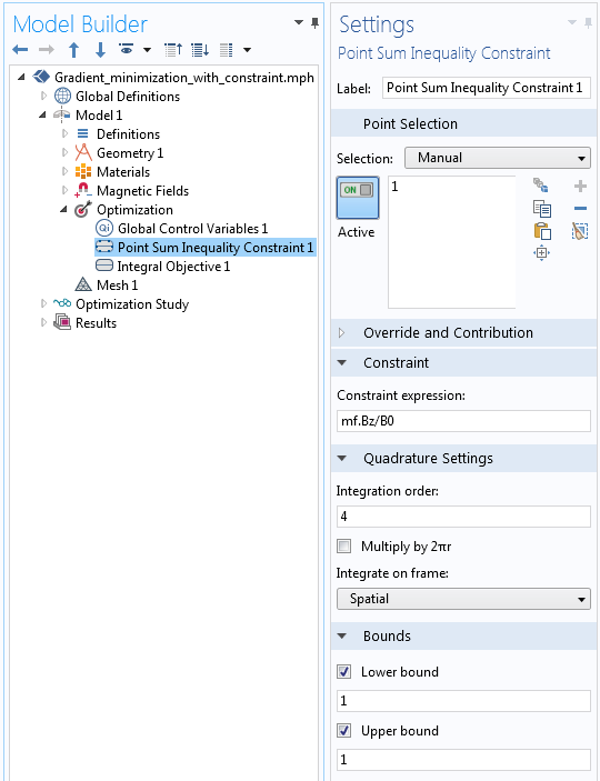
The implementation of an equality constraint.
The objective of minimizing the gradient of the field within the target zone is implemented via the Integral Objective feature (shown below). The gradient of the Bz-field with respect to the z-direction is taken with the derivative operator: d(mf.Bz,z).
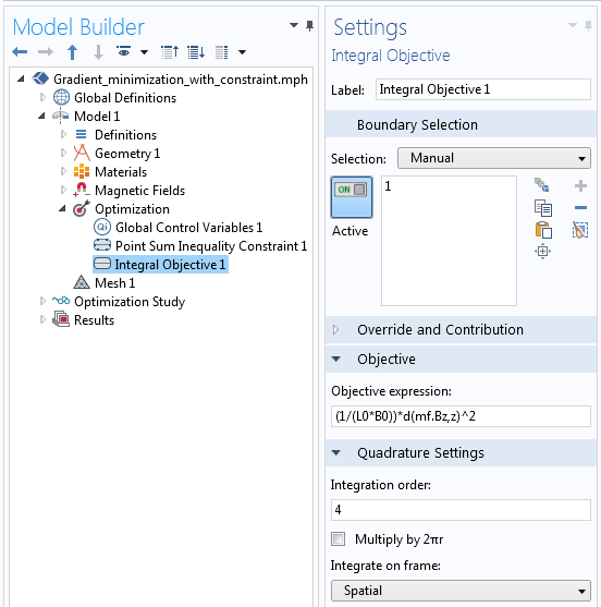
The objective of minimizing the gradient of the field.
We can use the same solver settings as before. The results for this case are shown below. The field within the optimization zone is quite uniform and matches the target at the centerpoint.
Results of optimizing for a minimum field gradient with a constraint on the field at a point.
Although the field here appears almost identical to the first case, the solution in terms of the coil currents is quite different, which raises an interesting point. There are multiple combinations of coil currents that will give nearly identical solutions in terms of minimizing the field difference or gradient. Another way of saying this is that the objective function has multiple local minimum points.
The SNOPT optimization solver uses a type of gradient-based approach and will approach different local minima for different initial conditions for the coil currents. Although a gradient-based solver will converge to a local minimum, there is no guarantee that this is in fact the global minimum. In general (unless we perform an exhaustive search of the design space), it is never possible to guarantee that the optimized solution is a global minimum.
Furthermore, if we were to increase the number of coils in this problem, we can get into the situation where multiple combinations of coil currents are nearly equivalently optimal. That is, there is no single optimal point, but rather an “optimal line” or “optimal surface” in the design space (the combination of coil currents) that is nearly equivalent. The optimization solver does not provide direct feedback of this, but will tend to converge more slowly in such cases.
Closing Remarks on Optimizing Current in Electromagnetic Coils
We have shown three different ways to optimize the currents flowing through the different turns of a coil. These three cases introduce different types of objective functions and constraints and can be adapted for a variety of other cases. Depending upon the overall goals and objectives of your coil design problem, you may want to use any one of these or even an entirely different objective function and constraint set. These examples show the power and flexibility of the Optimization Module in combination with the AC/DC Module.
Of course, there is even more that can be done with these problems. In an upcoming blog post, we will look at adjusting the locations of the coil turns — stay tuned.
Editor’s note: We have published the follow-up post in this blog series. Read it here: “How to Optimize the Spacing of Electromagnetic Coils“.
Further Resources
- Browse the COMSOL Blog for more information on modeling electromagnetic coils:


Comments (2)
Ivar Kjelberg
April 11, 2017Hi Walter
thanks again for a great Blog illustrating several impressive and advanced optimisation possibility with COMSOL.
A pragmatic practical engineering approach, to smoothen the field, would be to have the same current in all coils and optimise their individual axial position, another type of optimisation, on the geometry, that can just as well be done with the Optimisation module of COMSOL 😉
Sincerely
Ivar
Sergey Kuznetsov
September 25, 2018Hi Walter! I was wondering I you can comment on what is the best way in Comsol to add structural analysis in the coils and consider stresses and deformations generated in current-carrying structures due to magnetic fields.